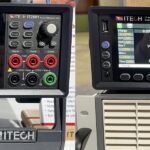
Test equipment is everywhere. Every trade show has it regardless of the focus. Power is no exception. At APEC 2024, EE World visited several booths displaying test equipment: meters, oscilloscopes, source-measure units (SMUs), bench power supplies, and electronic loads. The photos and videos below highlight what we saw, presented in alphabetical order by company. In […]
Analyzer
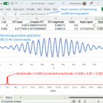
Why does the Fourier transform provide apparently inaccurate results, and what can I do about it? Part 4
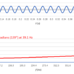
The FFT can measure phase angle, but what appears to be a meaningful result might just be the arctangent of a ratio of rounding errors. Throughout this series, we reviewed the fast Fourier transform (FFT) as implemented in Microsoft Excel and investigated windowing functions. In this final part, we’ll cover phase measurements, but first, let’s […]
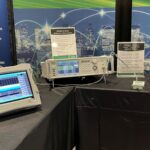
Perform phase noise and VCO measurements to 50 GHz
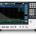
Rohde & Schwarz bumps up the frequency with the FSPN50 phase noise analyzer and VCO tester.
Wi-Fi 7 approaches, now comes the testing
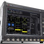
Keysight’s E7515W lets you test Wi-Fi 7 chipsets and systems.
Why does the Fourier transform provide apparently inaccurate results, and what can I do about it? part 3
Windowing functions account for mismatches between an input signal and FFT sample size. We concluded part 2 of this series with a look at fast Fourier transforms (FFTs) of 39.1-Hz and 38.12-Hz cosine waves, with our sample size N = 512 and our sample interval Δt = 1 ms (Figure 1). Shouldn’t the amplitudes of […]
AOC 2023: Exhibits show the latest in military wireless
Washington — The Association of Old Crows (AOC) held its 60th annual convention in Washington during the week of December 11, 2023. EE World was there on December 12. Here is some of what we saw in the exhibit hall. AOC is a defense-oriented conference that focuses on military wireless communications. In addition to product […]
TinySA Ultra: A low-cost spectrum analyzer that fits in your pocket

This palm-sized, battery operated instrument can help you diagnose EMC problems.
Audio analyzer combines analog and digital domains

The APx516B from Audio Precision comes with built-in analog I/O and a slot that adds wired or wireless digital I/O. With so many of today’s devices having audio capabilities, engineeers designing wired or wireless audio into a device need to verify audio quality. Audio Precision, well known for its audio analyzers, has introduced the APx516 […]
How do I choose an electric motor, and how do I test it? part 3
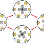
Motors follow the path of less reluctance to rotate. Thus, you need timing of applied power to get them moving. Part 1 and Part 2 of this FAQ looked at brushed and brushless DC motors, permanent-magnet and wound-rotor synchronous motors, and induction motors. These motors all have drawbacks, including mechanical wear of commutators, slip rings […]
What’s the difference between a PCIe analyzer and jammer?
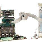
Protocol analyzers and jammers let you test and troubleshoot the performance of PCIe interconnects. From generation to generation, PCIe speeds double. Today’s protocols can be challenging to test and qualify. In addition, advanced applications such as the non-volatile memory express (NVMe) solid-state drive (SSD) memory protocol developed specifically for use with PCIe require sophisticated testing […]
