The first oscilloscope was derived from an apparatus involving a moving pen that recorded a change in voltage on a turning drum or paper strip. The first scope was a quite simple piece of equipment. Its heart was the cathode ray tube (CRT) equipped with vertical and horizontal deflection plates that caused an electron beam to move so as to produce a visible trace on a phosphor screen. The signal under investigation was applied to the vertical deflection plates to move the beam up and down displaying amplitude, and the horizontal deflection plates were used to create a time base.

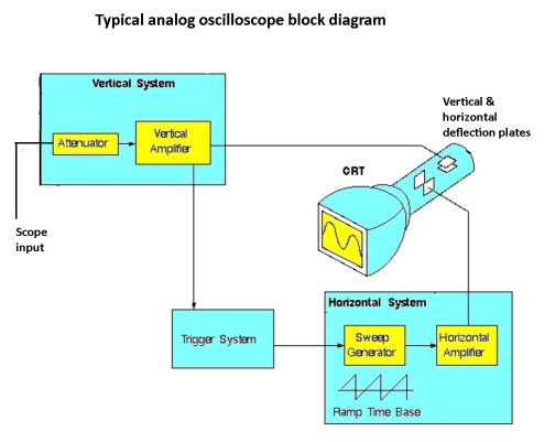This arrangement worked for non-recurring waveforms such as the human voice. For recurring periodic waveforms, these early machines were unsatisfactory; when the trace exceeded available horizontal space in the screen and reverted back to the left side, the successive wave cycles did not coincide. This confusing display can be simulated in a modern scope by raising the triggering level until it exceeds the highest peak voltage of the signal. The display then loses triggering and becomes incoherent.

This changed in 1946 when Howard Vollum and coworkers at Tektronix introduced triggered sweep in the Model 511 oscilloscope. The great innovation was that successive cycles initiated at the same point on the waveform, and in the display, as the oscilloscope triggered on a user-selected or default level of the rising or falling wave. The outcome was a coherent trace from which useful information could be derived.

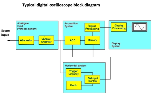The next great innovation was the internal structure of the LeCroy Digital Storage Oscilloscope (DSO). This instrument was somewhat more complex than earlier oscilloscopes, but the interface was quite user-friendly. The DSO is generally accompanied by the flat-screen display. The CRT is mostly obsolete except for a small number of educational units that are still sold. DSO and flat-screen technology make for a far more complex architecture in the modern oscilloscope. Semiconductor reliability and well-designed cooling eliminate most potential points of failure, but in the event of malfunction, even advanced electronics technicians generally send the units back to the factory for servicing.

Nevertheless, it is in the interest of technical professionals to examine the instrument’s internal electronics, particularly the signal flow, so as to understand processing and display functions. Most oscilloscopes are available in two- or four-channel models and occasionally more. Other than bandwidth, the number of channels is the foremost factor in determining cost.

The analog channel inputs sit on the front panel or, in many hand-held battery-operated models, these ports are on the top. A widely-used type of input accepts the BNC cable, which can attach to an AFG output on the rear or front panel, or to another instrument. These inputs also accept the output cables from the many types of probes that are available, having specialized tips that facilitate signal extraction from circuit boards and all sorts of terminals. The probes have various attenuation factors such as 10:1, and this extends the instrument’s range and protects against overvoltage.

The input impedance of the oscilloscope is high, typically 1 MΩ, although it can be reduced by the user for special measurements. The high impedance has the effect of mitigating loading in the circuit under investigation, so the oscilloscope is essentially invisible.

Because the DSO is digital, each analog channel contains an analog-to-digital converter (ADC). Subsequently, the now digitized signal is conveyed to memory. In the process, there is a complex interplay between memory depth and the sampling rate. It would seem that a greater memory depth would be advantageous, but this is not always the case, depending upon the application.

Despite the benefits of deep memory, it becomes problematic when the oscilloscope is unable to keep pace with its demands upon the system, so there is a slow update rate. As a consequence, there is the possibility of dead time, raising the possibility of missing important anomalies. But a fast update rate tends to mitigate the dead time that results when an oscilloscope has difficulty fulfilling the demands of its own deep memory.

The latest DSOs have capabilities such as built-in math functions that were unavailable in analog versions. They can add, subtract, multiply and divide two signals fed into separate channels, as well as compute the fast Fourier transform of the incoming signal, creating a frequency domain view that expresses signal amplitude as the amount of power going into specific points of the spectrum. It can be viewed alongside and correlated to the usual time domain display.

A Mixed Signal Oscilloscope (MSO) permits the viewing of both these waveforms in real-time juxtaposition to some other input signal. For example, it might be beneficial to view the output of the power supply juxtaposed with the signal flow to check fo any temporally concurrent faults, thus exposing a malfunction or product deficiency.

Other aspects of the DSO represent significant advances beyond the all-analog oscilloscope. For example, signals can be saved in nonvolatile memory and survive even after the instrument has been powered down. They can also be saved to a flash drive, transferred to a computer, emailed to colleagues or printed for distribution to students. All this thanks to the fact that digitized signals are capable of being stored and processed.

Of course, the CRT in old analog oscilloscopes was capable of rendering a crisp and accurate trace, but it has been rendered obsolete by the ubiquitous flat screen. The CRT was a power-hungry heat furnace, much too bulky and heavy to have a place in hand-held, battery-powered oscilloscopes.

The flat screen is a great advance for reasons besides the fact that it makes scopes lighter and more compact. Rather than a transparent overlay that was known as a graticule, the flat screen has an electronic grid showing divisions and ticks. The user no longer need count physical marks to estimate amplitude, time and frequency values. Instead, using the Measure function and pressing a contextual key lets the user see an exact rendering of the quantity in question.