Compensating Scope Probes: Old Way and New Way

By David Herres

EEs all know that any load is characterized by its impedance, which consists of resistance and capacitive and/or inductive reactance. These latter stand in opposition to one another. The lesser is subtracted from the greater and the result is combined with resistance to obtain impedance in accordance with the equation:

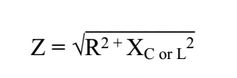
Where Z= impedance, Z; R = resistance, Ω; X_C or X_L = capacitive or inductive reactance.

As the equation suggests, resistance and capacitive or inductive reactance are not simply added to find impedance, but instead are combined vectorially. Impedance is equal to the square root of the sum of the squares. This rather oblique computation is necessary because resistance and reactance are pulling in somewhat different directions, like two oxen hitched to a log pulling at somewhat different angles. The net force results from their combined effort.

Resistance is constant for a given load, but reactance varies with the applied frequency. For an inductance, it is greater at a higher frequency, and for a capacitance it is greater at a lower frequency. In a transmission line, inductance is usually in series and capacitance is usually in parallel. In this case, both reduce the power transferred to the load, to a greater extent at a higher frequency.

All of this is applicable to a load, but it is equally applicable to the power source. Any battery, generator or signal source will have some amount of internal impedance, sometimes slight and sometimes great. The internal impedance acts as though it were external to the source and connected in series with it. Maximum power transfer takes place when source and load impedances are equal. This is a natural consequence of Ohm’s law because when the load impedance is low with respect to the source impedance, the circuit voltage declines. When the load impedance is high with respect to the source impedance, the current declines. Either way, there is less power transfer than if source and load impedances match.

When a signal is to be observed on the oscilloscope display, the probe becomes the source and the oscilloscope is the load. Due to slight variations, each probe must have its impedance matched to the respective channel.

To facilitate this process, modern oscilloscopes have external terminals where an internally generated square wave is available. To compensate a probe, plug it into a channel and connect the ground lead and probe to the correct terminals, which are labeled. Push Default Setup and Autoset. A square wave should be seen on the display. If it is not, the probe connections are probably at fault.

If you see the square wave drifting horizontally across the screen, adjust the trigger level to stabilize the display. Unless the probe and oscilloscope impedances happen to coincide, the square wave will be seen to be deformed with rounded corners. This is because the abrupt transitions at the rising and falling edges consist of rapidly changing voltages. The transitions are not accurately displayed due to the less than ideal power transfer.

The impedance of the probe can be adjusted to create a good match. The old way to do this was by using a non-metallic screwdriver to make an adjustment on the probe. A newer oscilloscope such as the Tektronix MDO 3000 series, does this for you when you follow the onscreen prompts. Probe compensation status is reported on the screen. Push the Menu Off button and you are ready to go. If there are separate probes for each channel, compensate each combination and label the probes.

Probe compensation is a simple task, but it must be done to get meaningful oscilloscope displays at any significant frequency.