Displaying signal jitter on an oscilloscope

A priority in digital environments is speed. High-bandwidth electronic equipment requires high-frequency clock signals. If the system is to function correctly, the signals must be timed accurately. What this means is that the successive rising and falling edges must happen at the proper point in each cycle.

Timing error is known as jitter. A small amount can be tolerated, but jitter above a critical level will cause bit errors. Jitter that is bad enough can cause complete signal failure. Jitter can be defined in several ways. Absolute jitter
is the absolute difference in the position of a clock’s edge from where it would be ideally. Period or cycle jitter is the difference between any one clock period and the ideal or average clock period. Cycle-to-cycle jitter is the difference in duration of any two adjacent clock periods.

All these definitions involve short-term variations, and “short term” here has a technical meaning. Long-term variations are known as wander, and the generally accepted boundary between the two is 10 Hz. Wander may be more easily mitigated than jitter. In serial communications links, a clock recovery circuit controls wander so that it does not degrade the signal.

Timing information may be conveyed by means of voltage transitions, changes in light intensity, or variations in air pressure as in acoustical phenomena. Any of these as well as other modes can be easily converted to electrical data by means of appropriate sensors and transducers. An oscilloscope can sample the changes in voltage (or occasionally current) so jitter analysis can proceed.

A few years ago, slower signaling rates meant less jitter, but increasing system demands have resulted in closer rising and falling edges, accentuating problematic jitter. Moreover, system voltages have been reduced, partly as an energy saving strategy and additionally to permit use of smaller batteries in small devices such as cell phones. Consequently, more compact waveforms with respect to X- and Y-axes are prone to a greater proportion of jitter.

Jitter is one among many types of noise, but it is particularly damaging in digital transmission. Because it involves deviations of clock edges from their correct location along the X-axis in an oscilloscope’s time domain, it can cause ones and zeros to lose their identities, thereby garbling the digital signal. Because of the cliff effect, digital transmission can successfully deal with several types of noise. But in regard to jitter, the best approach must be to eliminate the causes. Defects may be in the digital device or in the cabling that connects transmitter and receiver.

By placing an oscilloscope in the infinite persistence mode, it is possible to create an eye diagram that will reveal whether or not jitter exceeds an acceptable level. Period jitter is the simplest determination that can be made, and it is discerned by setting the oscilloscope on infinite persistence. Because successive peaks of the signal do not happen at the precise correct intervals, the distortion will be apparent. The instrument should be set to show slightly more than one complete clock cycle. As the oscilloscope triggers on the first edge, the period jitter shows up in the imperfect alignment of the second edge.

Cycle-cycle jitter may be quantified by looking at clock period change between successive cycles. This form of distortion can be ascertained by finding the actual difference in position of two cycles as opposed to merely noticing that they do not coincide.

These two types of jitter can be identified without reference to ideal locations of a reference clock, which many times is not available.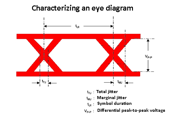

TIE (timing interval error) measurements, in contrast, are referenced to ideal locations of a clock signal. The assumption is that these ideal edge positions are known. Therefore TIE measurements cannot always be inferred by examining the oscilloscope display of an actual signal. The period jitter must be integrated after deducting the ideal clock period from each period of the signal as observed. The effects of TIE are cumulative. Eventually, the error reaches one-half the value of the waveform of interest, whereupon the eye is closed and correct communication isn’t possible.

All signals contain some degree of jitter. In evaluating a new prototype, one of the tasks is to quantify the amount of jitter and to find out if it is going to be problematic. To characterize jitter, statistical methods must be used. These include mean value, standard deviation, maximum, minimum and peak-peak values and population.

The mean or average level of a clock period may be taken as the nominal period. It is the reciprocal of the frequency. The TIE mean value is zero.

The standard deviation is the average amount that a measurement deviates from the mean value. It is represented by the Greek letter sigma (σ). Where the distribution is Gaussian, the amount at any point can be found by imputing the mean and the standard deviation. The peak-peak value is the minimum amplitude level subtracted from the maximum level.

The population is the total number of individual observations. Because the process is random, greater accuracy arises by taking more observations, i.e. acquiring a larger population. The object of the exercise is to reduce measurement uncertainty, and the population necessary should be ascertained by considering the qualities of the distribution.

To organize the information as outlined above, the tool of choice is the jitter histogram. Histograms are used in a wide variety of diverse applications, from census bureau data analysis to color saturation in digital cameras. Essentially, histograms are graphical representations of the distribution of numerical data. Implicit therein is an estimate of the probability distribution of a continuous quantitative variable. As such, no information is given about the order in which the observations were made.

A histogram can be created to depict a TIE measurement. Particularly where the pattern is repetitive and modulation or other periodic components are the object of inquiry, it may be necessary to go beyond the histogram and develop a plot of jitter values with respect to time. Once the pattern is acquired, its correlation with coupled noise can often be revealed.

Having plotted jitter measurements on X- and Y-axes in the time domain, it is a simple operation to do a Fourier transform so as to display the signal in the frequency domain. The Y-axis now measures amplitude as power on a logarithmic decibel scale, and the X-axis measures frequency. So the display shows various portions of the spectrum, as chosen by the user.

The analysis can take place on a spectrum analyzer, which has a large ensemble of analytic tools. A reasonably high bandwidth that is FFT-enabled will certainly suffice. Either way, spectral analysis will reveal periodic phenomena that would be difficult to see in a conventional time-domain display because it would likely be obscured by noise that exists across the spectrum. Random noise, in the frequency domain, is confined to the noise floor rather than appearing as waveform distortion in the time domain. After establishing a limit to the amount of jitter that can be tolerated, this noise floor can be measured across the spectrum.

An eye diagram will reveal at a glance the amount of jitter in a signal. However, to characterize the nature of a particular instance of jitter or when multiple varieties combine to derange a signal, numerous tools must be deployed, and a comprehensive analysis is needed before product redesign or prototype repair can reduce the jitter to an acceptable level if not eliminate it altogether.