A typical computer contains at least two separate memory substructures: random-access memory (RAM) and read-only memory (ROM). The digital storage oscilloscope (DSO) also has two types of memory: acquisition and display memory, but beyond that the comparison is tenuous.

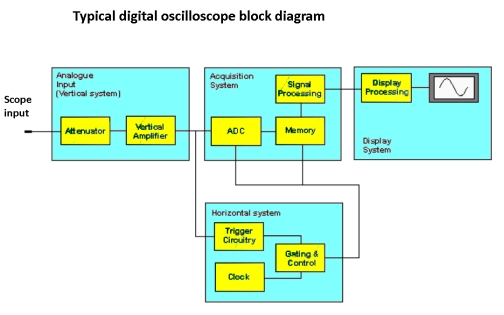In talking about a DSO, memory generally refers to acquisition memory. The highly complex interaction between acquisition memory and the central processing unit (CPU) takes place at awesome speed, whereas the display memory, in conjunction with user-controlled buttons and soft keys, is tasked only with delivering a finished product to the flat-screen display.

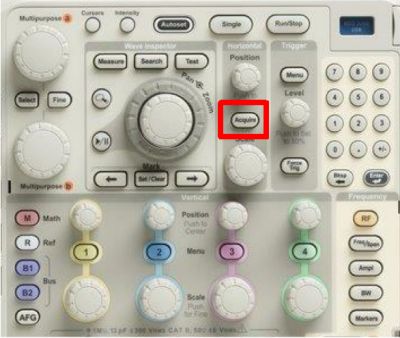
An important parameter in acquisition memory is record length or memory depth. For any given oscilloscope there is a maximum memory depth. This is one of the scope maker’s banner specifications. It is, however, sometimes desirable to adjust it down. To do this, in the Tektronix MDO3000 series oscilloscopes, press Acquire. The acquisition modes, shown in a vertical side menu, are Sample, Peak Detect High Resolution, Envelope and Average. In all of these modes, memory depth can be adjusted. This is done by pressing the soft key associated with Record Length in the horizontal menu at the bottom of the display. A vertical side menu appears with six alternate memory depths expressed in Record Length (points), one of which can be selected by turning Multipurpose Knob a.

In any discussion of memory depth, we must be cognizant of the sampling mode. The most fundamental and default of the various modes is known quite simply as sample mode. Like the other modes, it is characterized by the locations within the waveforms at which samples are taken.

In Sample mode, one sample is extracted and placed in the acquisition memory for each sample interval. Other potential samples are discarded in an action known as decimation. The procedure works well in most applications, but there are situations where critical (short duration, transitory) events are not available for display.

An effective solution is the Peak Acquisition mode. The highest and lowest peaks that occur in adjacent pairs of sample intervals are placed in the acquisition memory. Accordingly, glitches consisting of high and low values are revealed and can be evaluated at any point in the future, even after the signal is no longer connected to an oscilloscope input.

Acquisition metrics depend on the definitions and mathematical relationships among various sampling parameters. The sample interval is determined by the analog-to-digital converter (ADC) in conjunction with the clock. The sample interval is designated by t_S, in fractions of a second.

The amount of memory (record length) depends upon the sample rate and time duration of the waveform, as determined by the user’s choice of horizontal setting, which equates to units of time-per-division. The standard number of horizontal divisions is 10. If a given oscilloscope has a sample rate of 1 GHz and the horizontal scale is 20 μs/div, then the required memory is 200,000 samples (points).

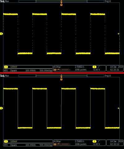
For a specific sample rate, required memory length is large for long time durations. This difficulty can be mitigated by reducing the sample rate. One of the sampling modes, High Resolution, reduces the sampling rate by averaging all sample points within a sample interval to create a single sample point. Like waveform averaging, the technique effectively limits noise, but it has the disadvantages of reducing bandwidth and hiding glitches. A plus is that vertical resolution is improved.

After these and/or other operations have been completed, the waveform is placed in memory. Next on the agenda is to display it. However, there is a potential conflict that must be resolved. A flat-screen scope display has typically 1,000 available pixels horizontally, so how is it possible to display an entire waveform whose full record may consist of millions of points?

This task is usually accomplished by compressing the samples to fit the flat screen. How is this possible given limited flat-screen resources? Some of the display points of necessity must coincide, and where they do, the relevant portions of the trace are rendered in progressively warmer or cooler colors (depending on how preferences are set) to indicate the waveform properties.

Segmented memory in an oscilloscope is an acquisition mode that is essential when measuring low duty-cycle events including laser communication, radar and sonar bursts and packetized serial bus data. The problem is that memory depth in available oscilloscopes is insufficient to capture and store the bursts plus the long dead time between them. Segmented memory permits the instrument to ignore the dead time and record only the actual waveforms and glitches that may arise between them.

A conventional solution for displaying low duty-cycle data was for the user to set the time base to an extremely slow time/division rate, but the problem was that the oscilloscope would compensate by reducing the sample rate. This lower rate degraded horizontal and vertical waveform resolution. Segmented memory came to the rescue.

The defining component in a DSO is the ADC. This function, usually within an integrated circuit rather than a discrete component, samples the analog waveform at specified intervals with reference to an external clock and conveys to the oscilloscope memory a digital number that denotes the signal’s amplitude at a point in time.

We know intuitively that a certain minimum number of samples must be taken to accurately render the signal. Accuracy in this context means that the digitized signal could be converted back to the original analog version and it would be a perfect match. In fact, you could go back and forth any number of times with no distortion or loss of information, subject only to a small amount of noise that might be introduced.

The Nyquist-Shannon sampling theorem states that perfect reconstruction of a signal with finite bandwidth is possible if the number of samples per unit of time is twice the frequency of the highest component. For a pure sine wave, which has no energy outside the fundamental, the sampling rate is simply twice the frequency of the signal. A non-sinusoidal signal, however, contains oscillating energy that exists as separate sine waves at discrete frequencies above the fundamental.

Thus, for perfect rendering of a non-sinusoidal analog signal into the digital version, the sampling rate must be based not on the frequency of the fundamental, but on the highest frequency in the signal’s spectrum. Therefore, the sampling rate of a non-sinusoidal waveform is dependent not only upon its center frequency but also upon its complexity.

Of course, what we want to see on the oscilloscope screen is an analog representation of the original analog signal at the oscilloscope input, not just a string of 1s and 0s. This is where, post-processing, digital to analog conversion (DAC) enters the picture.

In most applications, DACs exist as integrated circuits, but because they are required to operate at very high speeds, DACs in DSOs are likely to be discrete components. Regardless, the way they work is essentially the same. A DAC converts a digital data stream into an analog voltage that is suitable for display. The first step is to latch each voltage until the next one arrives. This has the advantage of filling in the gaps, but there are numerous harmonics that are above the Nyquist frequency, so they must be removed by means of a suitably calibrated low-pass filter.

Then, better interpolation is needed, and this varies with the nature of the signal. The most common interpolation method used in contemporary DSOs is sin(X)/x, as opposed to linear or pulse, and this interpolation method is preferred because it creates a trace curve that best captures the intent of the original waveform as it exists at the oscilloscope analog input.