Engineers should measure and analyze power integrity on the power and ground planes of a board’s power distribution network. Understanding power integrity is crucial when evaluating circuit power quality because it has a direct influence on performance.
Power integrity is a subset of signal integrity, whose assessment ensures that signals have suitable amplitude, rise time, noise, transient, and other characteristics for proper circuit performance under all operating conditions. Power integrity focuses on these same characteristics for the power distribution network (PDN) power rails to ensure that devices receive supply voltages that fall within the device’s specified operating ranges under all circuit operating conditions. Measurements play a significant role in power integrity.
Supply voltages in the PDN must be kept within a specified tolerance of their nominal value. A PDN’s noise, droop, and transients also need tight control. Cumulatively, this might mean an allowable power-rail variation of less than 1%, depending on the circuit. Therefore, a 1 V power rail might need to have variations in the rail voltage limited to ±10 mV (or less). Moreover, the bandwidth of the noise and transient signals on the power rail can extend beyond 1 GHz. Measuring the small (millivolt) variations of the power rail at relatively high bandwidths can prove challenging.
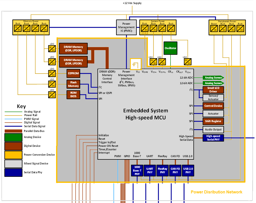
Figure 1 shows a typical embedded system. Its PDN includes voltage regulator modules (VRMs), low dropout (LDO) regulators, board interconnects, PCB power and ground planes, and bulk decoupling capacitors. Packaged semiconductor devices have internal power rails not shown in Figure 1 and are the focus of additional on-die power integrity analysis.
Noise and transients encountered in power-integrity measurements arise from many sources. Self-aggressive noise can arise from VRM to VRM, or the noise could originate at a processor core, I/O signals, or the VRMs. Mutual crosstalk between any of the circuit elements may also contribute.
When making power-integrity measurements, your goal is to assure the voltage levels of the rails (regulation) and to characterize the noise on the rails (e.g., ripple, droop under transient load conditions, pollution from other sources, etc.). Figure 2 shows an example of typical power-integrity measurements.
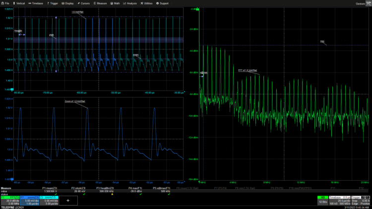
This analysis of a 1.5 V rail uses automated measurements to find the mean rail voltage and the peak-to-peak noise amplitude. A Fast Fourier Transform (FFT) lets you view the rail’s frequency spectrum. The frequency-domain view is a useful tool for analysis and troubleshooting. Most oscilloscope manufacturers create a dedicated spectrum analyzer user interface within the oscilloscope.
The key oscilloscope specifications relevant to power-integrity measurements are amplitude resolution, bandwidth, sample rate, vertical offset range, and memory length.
Amplitude resolution specifies the smallest amplitude difference in the acquired waveform that the oscilloscope can resolve. It is usually specified in terms of the number of bits of the oscilloscope’s digitizer. Assume you’re measuring 5 mV of ripple or noise riding on a 1 V rail. The ripple voltage is 46 dB (200:1) lower than the rail amplitude. A rule of thumb is that an oscilloscope’s theoretical amplitude dynamic range is 6 dB per bit. An 8-bit oscilloscope may have a usable dynamic range of 48 dB (at best), while a finer-resolution oscilloscope will have a wider dynamic range. This difference appears in the comparative signal clarity of the two captures in Figure 3.

An oscilloscope’s bandwidth limits the range of frequencies that the instrument can measure. While the rail signals are nominally at DC, rail noise and transients can have a wide frequency range. In general, PDN power-integrity measurements require oscilloscope bandwidth from 500 MHz to 2 GHz to accurately capture noise and transient events on the board-level power rail, with even more bandwidth required to measure closer to or on the die rails.
An oscilloscope’s maximum sample rate must be greater than twice its bandwidth. Most modern instruments have minimum oversampling of four or five times the bandwidth, and this increases the horizontal (timing) resolution and the ability to accurately capture high-speed transients. The sample rate also sets the upper-frequency limit of the FFT at half the sampling rate.
The vertical offset range sets the maximum vertical sensitivity you can use to measure a power rail, depending on the probe you use. The oscilloscope’s offset shifts the DC rail voltage and centers the power rail signal vertically on the oscilloscope grid. Adjusting the oscilloscope’s gain sensitivity to 10 mV/div or less lets you view small amplitude changes on the power rail. A typical oscilloscope may have 1 V of offset (or less) at the highest sensitivities (e.g., below 100 mV/div or 50 mV/div) — not enough to center the power rail and view transients at the highest sensitivities. Oscilloscopes optimized for power-integrity measurements provide enough offset at higher sensitivities to not limit rail measurements. Furthermore, attenuating probes, such as the 10:1 passive probe supplied with your oscilloscope, restrict the instrument’s offset range because the probe’s attenuation factor shifts the oscilloscope-plus-probe combination offset range by the attenuation factor.
An oscilloscope with an offset specification of 1 V at 5 mV/div will, for example, be restricted to 1 V of offset at 50 mV/div (10 times 5 mV/div) when using a 10:1 passive probe. This restricts the highest sensitivity gain setting that you could use to view small voltage ranges. Using a home-built coaxial rail probe or a specialized power rail probe can minimize the impact of the offset range either by reducing the attenuation or increasing the offset range.
The oscilloscope’s acquisition memory length sets the record’s maximum duration, which is important for operations such as measuring power sequencing at startup and shutdown. Large amounts of acquisition memory can help you understand and debug complex cause-effect scenarios in an operational system when looking at many power rails at once. The maximum acquisition length also determines the FFT’s frequency resolution.
Probing options
Viewing power rails requires a probe. There are several considerations in the choice of an oscilloscope probe for power-integrity measurements. The first is that the signals of interest are often small voltages atop larger DC voltages, and the noise that the measurement system (oscilloscope plus probe) contributes must be smaller than the signals of interest. The oscilloscope-probe combination must have sufficient bandwidth to not alter signal components of interest. The PDN’s power rail may carry only a small amount of current, and the probe should not load the power rail (draw too much current in comparison to what it is designed to carry). Impedance differences between the probe and the PDN will also cause reflections of high-frequency components. Finally, the instrument system should have sufficient offset to match the rail voltage when the probe is connected.
The first probing option is the use of the 10:1 passive probe usually supplied with the oscilloscope. This passive probe uses a 9 MΩ resistor in series with the oscilloscope’s 1 MΩ input, forming a 10:1 attenuator. This attenuator is compensated by using a small capacitor in parallel with the 9 MΩ resistor, forming a high-pass filter that compensates for the low-pass characteristic of the oscilloscope’s input. An adjustable capacitor in the probe compensates the attenuator by making the high-pass and low-pass filter cutoff frequencies equal. Always compensate this type of probe whenever you connect it to an input channel.
An oscilloscope’s 10:1 passive probe has some limitations. The 10:1 attenuator reduces the input signal supplied to the oscilloscope input, which the oscilloscope must then scale back up. Therefore, the additive noise of the probe is ten times, or 20 dB, greater than the actual noise.
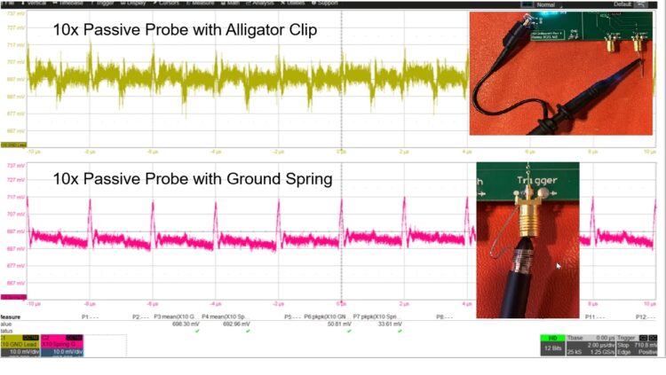
The 10:1 passive probe often comes with a variety of tip accessories for different interconnection methods, the choice of which can affect its performance. The most often used accessory is the spring hook, which uses a long ground wire terminated with an alligator clip. This combination works well for low-frequency signals — higher frequency measurements will incur noise because the probe’s ground wire forms an antenna through the ground loop. Instead, use a ground spring accessory, which employs a spring wrapped around the probe’s ground ring with a very short projection. This minimizes the high-frequency pickup. Figure 4 shows the variation in noise pickup for each method.
A coaxial connector adaptor accessory may also come with the passive probe, or you can purchase it from third-party suppliers. It can mount on the board, which reduces noise pickup.
You can also use 10:1 transmission-line probes that terminate into the oscilloscope’s 50 Ω input. These probes offer short leads and wide bandwidth (greater than 1 GHz). Like the 1 MΩ coupled 10:1 passive probe, the transmission line probe attenuates the input and increases internal noise scaled to the connection point. External noise pickup is low, but this type of probe has a lower input impedance of 500 Ω, which may cause loading problems.
You can also connect a 50 Ω coaxial cable directly to the power rail to use as a probe. There is no attenuation with this connection, so there is no additive noise. If the coaxial cable is terminated into the 50 Ω input of the oscilloscope, then the cable input is a 50 Ω load on the connection point. This can cause circuit loading problems, especially if the power rail supplies very small currents. For example, for a 5 V rail, the oscilloscope input would draw 100 mA, and this could be a considerable load current for a battery-powered device. Most oscilloscopes also limit the maximum voltage at the 50 Ω input to 5 V or less — make sure you don’t exceed this input limit or you could damage the oscilloscope’s input amplifier.
Using a coaxial cable terminated into the oscilloscope’s 1 MΩ input may work for low-bandwidth (below 500 MHz) measurements, but this arrangement will result in high-frequency reflections. If you can recognize the signature of these reflections (and ignore them in your circuit assessment), this may be a good, low-cost technique that minimizes loading and reduces additive broadband noise.
The final probing method is a power-rail probe. The power rail probe, as the name implies, is designed specifically for measuring power rails. It has a dual-path connection offering high input impedance (50 kΩ) at DC to minimize circuit loading and 50 Ω input impedance above 1 MHz Bandwidth is typically 2 GHz to 8 GHz, depending on the supplier. Its coaxial connections minimize pickup, with only small (nominally 1x) attenuation so that it doesn’t increase broadband noise by adding gain to an attenuated signal. The power rail probe has a built-in internal offset in the range of 24 V to 60 V. The downside of this probe is that it does cost more, but it is overall the best-performing solution.
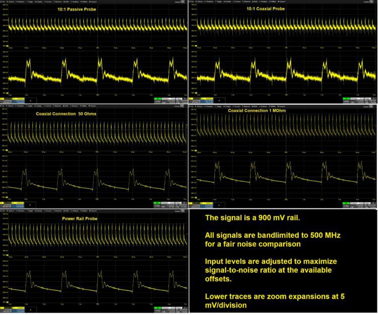
Figure 5 compares the performance of the five probing methods described above when analyzing a 900 mV rail. The coaxial connection at 50 Ω and the power rail probe provide the best signal integrity. Both 10:1 probes show additive broadband noise, as expected. The coaxial connection terminated into 1 MΩ shows the reflections of the fast edges due to the impedance mismatch.
Although the 50 Ω terminated coaxial connection produces excellent results at 900 mV, it has a limited offset range (requiring sufficient offset to be available in the oscilloscope) and potential loading issues due to its low impedance. If, however, the oscilloscope has sufficient internal offset and circuit loading is not a concern, this is a very low-cost and high-performance solution to probing a power rail.
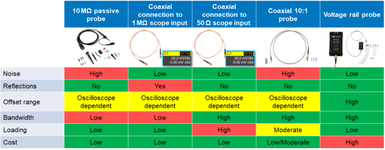
A summary of the probing options for power-integrity measurements appears in Table 1. With attention to specific situations, you can use any of these probing methods for power-integrity measurements. The power-rail probe offers the best performance under almost all conditions. Unfortunately, it’s also the highest cost.
Power-integrity software
Many oscilloscope manufacturers also offer specialized power integrity software to simplify the measurements, such as that shown in Figure 6.
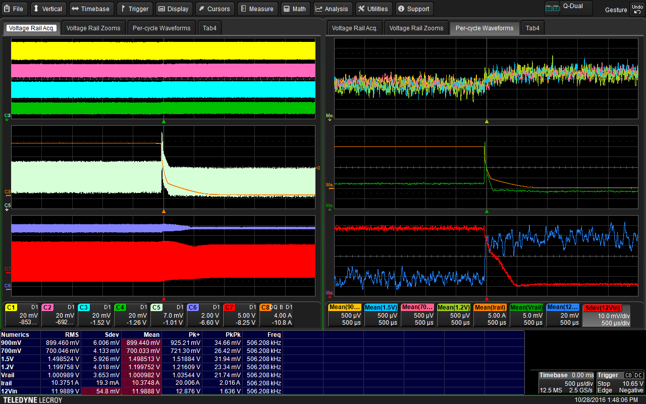
These software packages capture power rail signals over thousands of switching periods and display statistical data values of the necessary measurements. They also perform a cycle-by-cycle analysis of the rail voltages and plot the changes in rail voltage over time as per-cycle waveforms. This vividly displays the behavior of the power rails in a highly intuitive and useful manner.
Recommendations for making power-integrity measurements are listed below:
- Remember that it’s easy to make a measurement, but it is hard to make a measurement without artifacts.
- Know the capabilities and limitations of the probe you choose to use.
- If you chose to use a 10:1 probe, remember to use the low-inductance tips and adaptors.
- For the best performance, use a power-rail probe if cost is not an issue.


Leave a Reply
You must be logged in to post a comment.