In choosing a way to mitigate electronic noise mitigation, it is necessary first to quantify it and ascertain its source.
Thermal, also known as Nyquist or Johnson-Nyquist noise, is basis for many types of noise. It arises in all material objects to the extent that they are conductive. You can observe the effects of this noise by connecting a sensitive digital multimeter in volts mode to the leads of a resistor sitting on an insulated surface. When set to a sufficiently sensitive range, the instrument displays rapidly fluctuating values. Electricians call this “phantom voltage.” As soon as you lock onto a live source, the chaotic display stabilizes into a valid readout.
The noise power from a resistor depends on its temperature, resistance, and a specified bandwidth. The general form of the Johnson-Nyquist RMS noise equation for a resistor R becomes
![]()
where: k = Boltzmann’s constant (J/K), T = temperature in Kelvin (°C + 273.16), R = resistance in ohms, and B = bandwidth. Room temperature is about 290 K.
For a 1 kΩ resistor at room temperature and a 10 kHz bandwidth, the RMS noise voltage is 400 nV. A useful rule of thumb to remember is that 50 Ω at 1 Hz bandwidth correspond to 1 nV noise at room temperature.
A resistor in a short circuit dissipates a noise power P of
P = V2/R = 4kTΔf
The noise generated at the resistor can transfer to the rest of the circuit. The maximum noise power transfer happens with impedance matching when the Thévenin equivalent resistance of the remaining circuit equals the noise-generating resistance. In this case each one of the two participating resistors dissipates noise in both itself and in the other resistor. Because only half of the source voltage drops across any one of these resistors, the resulting noise power P in Watts is given by P = 4kTΔf. A point to note is that this quantity is independent of the noise-generating resistance.
We observe this thermal noise in the display of a spectrum analyzer or oscilloscope in FFT or RF mode. It appears as a rapidly fluctuating, roughly horizontal trace near the bottom of the screen. This is known as the noise floor of the instrument, and it has to be seen to be appreciated.
The frequency of thermal noise, besides being random, is not bounded. This means that, unless it is purposely limited, the bandwidth is infinite. On an oscilloscope, this noise makes a blurry trace, and a sufficiently noisy signal will lose triggering and eventually become unrecognizable. There is a simple mitigation technique, which consists of temporarily reducing the bandwidth (not of the instrument, but of the signal). If the bandwidth of a 1-GHz oscilloscope signal is limited to 50 MHz, for example, depending on the amplitude of the signal and the amplitude of the added noise, there may not be much effect on the display. But if you reduce bandwidth to 20 MHz, you’ll probably see a clean signal, characterized by a thin trace. The transformation is more striking in the frequency domain. A limitation of this technique, however, is that you can’t cut the bandwidth below the requirements of the desired application.
A few words about the Boltzmann constant: Denoted in equations as k, it is the proportionality factor that relates the average relative kinetic energy of particles in a gas to the thermodynamic temperature of that gas. In other words, as the heat goes up, the kinetic energy and thermodynamic temperature both go up, but the Boltzmann constant stays the same. The constant also plays a role in Planck’s law of black body radiation. It is a small number indeed. The Boltzmann’s constant is currently set at 1.380649×10⁻²³ J/K.
The amplitude of thermal noise depends upon the temperature of the conductor in degrees Kelvin and the total bandwidth under investigation. Noise power N (in Watts) is calculated according to N = kTΔf where Δf is the bandwidth in Hertz, T is the temperature in degrees Kelvin, and k is the Boltzmann constant. The resulting noise is in Joules/sec or Watts. To convert the noise power to dB·Watts, use 10 times the log of the noise power in watts. Assume room temperature is 290 K. The normalized (Δf = 1 Hz bandwidth) noise floor equation is
Noise floor = 10log(kTΔf) =10×log(1.38×10-23×290˚×1 Hz) = -203.9 dBW⁄Hz
Next, to convert from dBWatts to dBmilliwatts (dBm), increase this value by 30 dB:
–203.9 dBW⁄Hz+30 dB= -173.9 dBm⁄Hz
This is the amount of noise power in a 1 Hz bandwidth.

There are several ways to measure a circuit’s noise figure. One is called the gain method. To use it, the gain of the DUT must be known. The gain method uses the noise factor definition:
Noise Factor = (Total output noise power)/(Output noise due only to input source)
Here noise arises from two effects. One is the interference that comes to the input of a (typically RF) system. The second comes from the random fluctuation of carriers (i.e. Brownian motion) in the circuit from thermal effects. Starting with P = 4kTΔf , we get a room temperature power density of -174dBm/Hz. Then the noise figure NF of a DUT is NF = PNOUT – (-174 dBm/Hz + 10log(Δf) + Gain) where PNOUT is the measured total output noise power, -174 dBm/Hz is the noise density of 290°K ambient noise, Δf is the bandwidth of the frequency range of interest, and Gain is the system gain.
Then the input of the DUT is terminated with the characteristic impedance (50 Ω for most RF applications, 75 Ω for video/cable). One way to measure random noise in a circuit employs a noise source that introduces a known noise signal into the circuit of interest. If you know the noise power going into the circuit of interest, you can measure its output and calculate the device’s noise contribution to the circuit, called its noise figure. Then the output noise power density is measured with a spectrum analyzer.
Thermal noise also enters into calculations of an RF receiver’s sensitivity. Sensitivity can be calculated if one knows the noise figure (NF), the equivalent noise bandwidth (ENBW), and the carrier-to-noise ratio (C/N) needed to produce a desired signal quality:
Receiver sensitivity=10×log(kTB)+NF+C⁄N
This equation defines the signal power in dB·Watts that is present at the demodulator for a desired carrier-to-noise ratio.
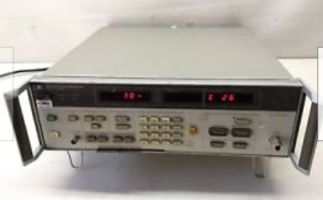
Several types of instruments can measure noise power as well as noise figure. A noise-figure meter resembles a conventional RF receiver but it has controllable bandwidth and an accurate power-level detector.
It’s also possible to use an ac voltmeter or a power meter to measure a UUT noise output power. In the case of using a voltmeter, the measured voltage and the circuit’s load are used to calculate noise power.
It is also possible to get a rough noise measurement with an oscilloscope that includes a phosphor persistence display mode. This technique uses two scope channels that both connect to the same point in the circuit. Both channels are set to the same range and put in alternate-sweep mode. The two traces are positioned vertically until there is a dark band between them. Then the position of one channel is adjusted until the overlapping noise from the two traces fills the dark band.

Next the signal is removed from both scope inputs by setting both channels to ground. Now just measure the distance (in graticule units per division) between the noise-free baseline traces. Multiply the distance by the volts/div settings to yield the circuit’s random noise.
Finally, a few other types of noise that arise in electronics. Shot noise is generally considered different than thermal noise though it also is based on non-periodic thermal fluctuations. Shot noise arises when electrons cross a gap. These and other charge carriers arrive at random and discrete intervals. The noise is likened to rain falling on a tin roof.
The root-mean-square value of shot noise σi is expressed in the Schottky equation:
![]()
where I is the dc current, A; q is the charge of an electron; and ΔB is the bandwidth in Hz.
Shot noise arises in vacuum tubes because electrons randomly leave the cathode and thus randomly arrive at the anode. Resistors and other conductors do not exhibit shot noise because the charge carriers, without discrete arrival times, move diffusely through the device. Only in the smallest resistor, where the size is less than the electron scattering length, is shot noise observed.
Flicker (i/f) noise is characteristic of a signal with an amplitude that falls off at higher frequencies. It is also known as pink noise. It is a property of electronic devices which, due to their series impedance and parallel capacitance, attenuate higher frequencies. Flicker noise is believed to be caused by charge carriers that are randomly trapped and released between the interfaces of two materials. The phenomenon is linear in resistors and FETs but non-linear in BJTs and diodes. Flicker noise is a function of the material homogeneity, its volume, the current, and the frequency. Popcorn noise, on the other hand, is proportional to 1/f2 and is associated with poor semiconductor manufacturing. It appears as a series of low-frequency noise bursts.
Burst noise was first observed in point-contact diodes and seen in the 709 op-amp. A common cause is the capture and release of charge carriers at their film interfaces.
Transit-time noise is generated when the time required for electrons to travel from emitter to collector in a transistor is close to the period of the signal being processed. It arises primarily at frequencies in excess of VHF. There, the noise impedance of the transistor drops until other sources of noise are obscured.


Leave a Reply
You must be logged in to post a comment.