Many oscilloscope users become adept at acquiring signals in the time domain and using Math>FFT in mixed domain oscilloscopes to display signals simultaneously in time and frequency domains. This is excellent for demonstrating the fundamental relationship between these different display modes, and the whole thing is user-friendly and intuitive.
In a Tektronix MDO3000 oscilloscope, at the far right of the front panel are five buttons and an input port which comprise the frequency or RF section of the instrument, and for users first working in this area, the controls and menu choices may seem somewhat recondite. But all this can be clarified.
By way of review, the groundwork for frequency domain as derived from a time-domain display of waveforms was established by Joseph Fourier. In the language of mathematics, Fourier found that any function (waveform) of a variable, whether continuous or discontinuous, can be expanded in a series of sines of multiples of the variable. This insight is the basis for transforming time domain into frequency domain of any given signal, known as Fourier analysis. The inverse, Fourier synthesis, is the process by which a time domain waveform can be derived from its frequency domain version.
For many decades, the mathematics for doing these transforms was complex and time-consuming. Then in the 1960s, a simplified set of algorithms known as the Fast Fourier Transform (FFT) emerged from obscure beginnings, permitting instantaneous transforms to be accomplished merely by clicking a computer mouse or pressing an oscilloscope button.
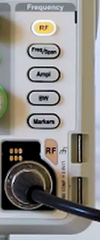
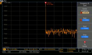
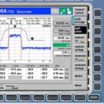
In the MDO3000, the top button in the Frequency section is RF. Pressing it turns off all analog channels. Math and AFG remain on. With no signal applied to the RF input, all we see on the screen is the frequency domain grid with a prominent, highly irregular, rapidly fluctuating horizontal trace about one-third of the way up from the bottom of the display. This is the noise floor of the instrument, caused by thermal activity and electron flow that is present in any conductor or device that is at some temperature above 0°K. Below this noise floor, no signal can be detected and consequently manufacturers constantly endeavor to lower the noise floor.
To see a waveform in the frequency domain, we must apply a signal to the RF input. A good source is the oscilloscope’s internal AFG, accessed by running a BNC cable from AFG Out on the rear panel to the RF input, equipped with an RF adapter. With the AFG on, the default sine wave displays in the frequency domain. It is difficult to see because the single spike that is the fundamental coincides with the left edge of the display.
We need to bring it to the center of the screen. To do this, first press Freq/Span, which is directly below RF in the Frequency section. The vertical Frequency and Span menu appears at the right of the display. Do not be distracted by the R to Center menu choice at the bottom. It has no relevance to what we are doing right now.
Take note of the AFG information bar at the bottom of the screen below the RF information bar. It informs the user that the current frequency of the sine wave is the default 100.00 kHz. Go back to the Freq/Span menu. Center
frequency is high, the amount determined by the oscilloscope model. It can be set by turning Multipurpose Knob a, but a lot of twirling can be avoided by using the keypad. Type in 100 and press the soft key associated with kHz in the Units menu that appears. Immediately, the sine wave fundamental moves to the center of the display where it can be clearly seen.
We can similarly display any of the available waveforms in the internal AFG. To do this, press AFG once more so the horizontal AFG menu appears across the bottom. Notice that the Freq/Span settings do not change. Press the soft key associated with Waveform so the vertical Waveform menu
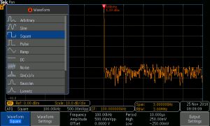
appears at the left. Use Multipurpose Knob a to scroll down to Square Wave. There it is in the AFG information bar with the 100 kHz frequency and 500.00 mVpp amplitude, both default values.
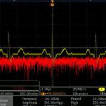
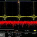
We know the square wave is a prodigious source of harmonics, due to the rapid rise and fall times, which are essentially high-frequency components. But these harmonics do not appear in the display. Where are they? For the answer to this question, go back to the Frequency and Span menu by pressing the Freq/Span button. As you can see, the span, 3.00 GHz, is way too large to display the harmonics, except for a little puzzling activity adjacent to the fundamental.
Press the soft key associated with Span and again using the keypad, try various values. One, five, ten and fifty MHz provide different perspectives.
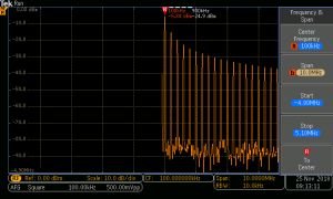
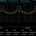
As you enter Span values, notice that Start and Stop frequencies automatically fall into line while Center frequency remains unchanged. The same situation happens when Start and Stop values are changed. Span automatically adjusts to conform to these new settings. You can press Menu Off to get a better view. Now we see an array of harmonics, evenly spaced and diminishing in amplitude as they get farther in frequency from the fundamental.
Most digital oscilloscopes and spectrum analyzers including PC-based instruments have similar Freq/Span controls and menus. Center Frequency, Span, Start and Stop may seem counter-intuitive at first, but soon this peculiar logic becomes clear.
The remaining Frequency section buttons more closely resemble time-domain controls.
Amplitude, accessed by pressing the third button from the top in the Frequency section, is helpful in creating a meaningful display. In many of the displayed AFG waveforms, the fundamental goes to the top of the screen, and you can’t tell whether it stops there or hypothetically goes beyond. In either event, the trace is difficult to read. Pressing Autoset may or may not resolve the situation. Intermittently a warning sign appears: Signal clipping, possible distortion.
Clipping in electronics arises when the amplitude of a signal rises above the capability of a circuit or component. In a sine wave, it is seen as a flat top of the waveform rather than the characteristic rounded peak.
When the RF Amplitude button is pressed, the vertical Amplitude menu appears at the right. The top menu choice is Ref Level, which can be adjusted by turning Multipurpose Knob a. The default reference level is 0 dBm, which puts the signal out of the display and into clipping territory. The most positive level is 20.0 dBm, which creates a good readable display. The number of dB per division can be adjusted by turning Multipurpose Knob b, which has the effect of moving the trace up or down in the display. These changes can be seen in the vertical scale on the left. Low is 1 dB/div and high is the default 10 dB/div.
Vertical units can be set by pressing the associated soft key and turning Multipurpose Knob a. Pressing the soft key associated with Auto Level bring the fundamental peak back to the top of the display.
Amplitude can also be changed by going back to the AFG and pressing the soft key associated with Waveform Settings, which bring up a vertical menu on the right. Pressing the soft key associated with Amplitude, we see that it can be changed from the default 500.00 mVpp by turning Multipurpose Knob a. Notice that this has no effect on the scaling. It is the actual AFG voltage that is changed at the RF input, as can be seen in the AFG information bar. The high voltage is 5 Vpp, which puts the fundamental out of the display and into the clipping range.

Leave a Reply
You must be logged in to post a comment.