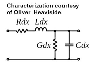
You can thank Oliver Heaviside (actually a short, thin man), for the telegrapher’s equations (or just telegraph equations). These are probably better known as the transmission line equations. They are actually a pair of coupled, linear partial differential equations that describe the voltage and current on an electrical transmission line with distance and time. RF reflection coefficients, VSWR, and a host of other common RF measurements all arise out of Heaviside’s transmission line model described in an August 1876 paper. The model demonstrated for the first time that electromagnetic waves can be reflected on a wire and that wave patterns can form along the line.

Originally developed to describe telegraph wires, Heaviside’s work also is applied to radio frequency conductors and antennas, telephone lines, power lines, and pulses of dc.

The telegrapher’s equations are actually a summation of Maxwell’s equations, more practical in that they assume the conductors are made up of an infinite series of capacitors, inductors and a distributed resistance. (Heaviside was a great simplifier.) The inductance and capacitance work in opposing ways with respect to frequency. Greater capacitance attenuates low frequencies more than high frequencies. DC passes through an inductor (except for its resistance component), while a capacitor permits flow of high frequency current.

We have to beware of the fact that in electrical circuits, inductive components are generally in series with the power or signal flow, whereas in capacitive circuits, the components are in parallel, Accordingly, in a transmission line, equal line segments balance out in terms of series inductance and parallel capacitance. That is how the apprentice can make sense of the enigma of characteristic impedance, i.e. for all given line lengths the impedance is the same, based on the characteristics of line design, which have to be carefully controlled during cable manufacture. Heaviside saw all this, and invented coaxial cable, for besides being a great theoretician and mathematician, he was an inspired electrical experimenter and builder.

In 1880, the year Heaviside patented coaxial cable, he researched the skin effect in transmission lines. Then came his major work, revising Maxwell’s mathematical analysis so that it conformed more to current usage and giving rise to vector terminology. This reduced twelve of the original twenty equations in twenty unknowns to four differential equations in two unknowns, as used today by electrical engineers.

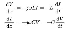
The Wikipedia page on the telegrapher’s equations does a good job of deriving the forms of Heaviside’s equations that are useful in various situations. Briefly, the basic equations themselves are

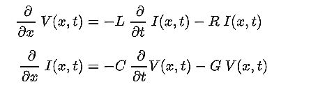
Here L, C, and R are inductance, capacitance, and resistance; G is conductance. The two equations can be combined to get two partial differential equations, each with only one dependent variable, either voltage or current.

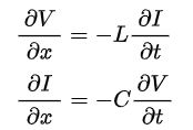
When ωL>> R and ωC>> G, wire resistance and insulation conductance can be neglected to yield an ideal transmission line considered lossless. In this case, the model depends only on the L and C elements. The telegrapher’s equations then describe the relationship between the voltage and current along the transmission line as a function of position and time.

The equations themselves consist of a pair of coupled, first-order, partial differential equations. The first equation shows that the induced voltage is related to the time rate-of-change of the current through the cable inductance. The second shows that the current drawn by the cable capacitance is related to the time rate-of-change of the voltage.

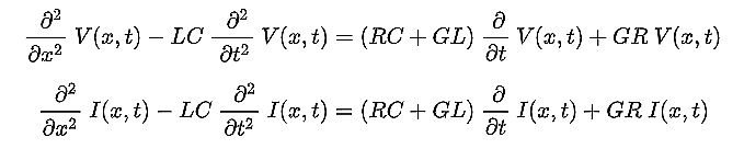
Combining the two yields two wave equations for voltage and current.

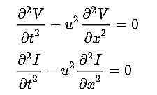
where u = 1/(√ LC) = the propagation speed of waves traveling through the transmission line.
When R and G are too big to neglect, the differential equations describing the elementary segment of line are

It was Heaviside who first saw coaxial cable as the solution for avoiding magnetic coupling that far outran the midcentury methodology. In a nutshell, Heaviside was a self-taught English scientist–and above all, a mathematician–who successfully combined imaginary numbers for the analysis of circuits, expanding our knowledge of conventional circuits as well. He also broadened our understanding of differential calculus and most important, developed circuit techniques that are used worldwide today.

This most profound work, currently applicable, for testing and instrumentation, he titled simply Electricity and Magnetism. It was published in the Journal Electricity in 1885.

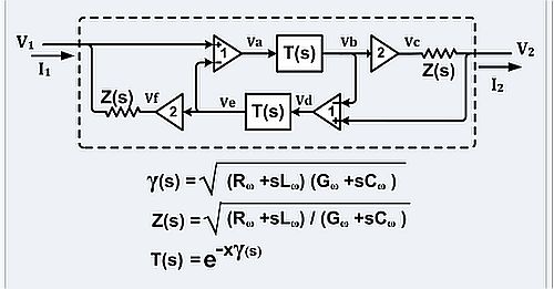Solutions of the telegrapher’s equations can be inserted directly into a circuit as components. One example found on Wikipedia is displayed here, but it is not unique and there can be many others. This example is that of an unbalanced transmission line such as a coaxial cable or microstrip line. Here 2/Z_o = transadmittance (The ratio of the change in output current to the change in input voltage across a circuit,) of a VCCS (Voltage Controlled Current Source), x ≡ length of transmission line, Z(s) ≡ Z_o(s) ≡ characteristic impedance, T(s) ≡ propagation function, γ(s) ≡ propagation “constant,” s ≡ j ω , j² ≡ −1 . The voltage doublers, the difference amplifiers, and impedances Z_o(s) account for the interaction of the transmission line with the external circuit.