The ideal capacitor consists of two conductive plates separated by a thin dielectric layer that separates and insulates the two plates from each other so they have no direct or resistive electrical connection. When voltage is applied across the plates, they store the electrical charge.
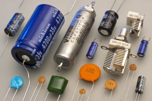 The capacitor may take many forms. If the plates are composed of flexible foil, they may be rolled into a compact cylinder that permits large-area plates in a small form factor. If low capacitance is required as in RF circuits, the plates may consist of two small electrodes embedded in a ceramic that serves as the dielectric layer.
Ideal capacitors are electrically defined by two parameters, capacitance and working volts. Working volts are simply the maximum voltage that can be applied to a capacitor without risk of creating an ionized path and making a permanent conductive path through the dielectric layer, destroying the component. In replacing a defective capacitor, you can generally go to a higher working voltage if it will fit in the space, but you cannot go to a lower working voltage.
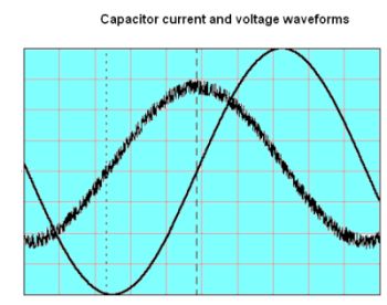
The opposition by a capacitor to the flow of current in a circuit is known as capacitive reactance. It varies inversely with the frequency of the applied voltage. If you look closely at a sine wave, the rate of change is greatest when the voltage is least and the rate of change is least when the voltage is peaking. The fact that a capacitive circuit responds not to amount of voltage but rather to rate-of-change accounts for phase shift, which may be observed in two oscilloscope channels, one using a voltage probe and the other a current probe.
An equation applicable to all capacitors is Q = CV, where the stored charges in coulombs on the two plates are Q and -Q, the capacitance in farads is C and the applied voltage is V.
The relevant equation for capacitive reactance is:
XC = 1/2πfC where XC = capacitive reactance in ohms; f = frequency of applied voltage in Hz; and C = capacitance in farads
When a capacitor is connected in series with a resistor and voltage applied across the combination, the capacitor will charge until its voltage approaches that of the source. And when the voltage is removed, it will decline, approaching zero. If the voltages in each case are graphed in the time domain, amplitude plotted against the familiar Y-axis and time plotted against the X-axis, the representations will be logarithmic non-linear curves, beginning steeply and leveling off as the endpoints are approached. The precise form or shape of these curves reflects the time constant of the resistor-capacitor combination. Any such configuration has a time constant, based on the capacitance and resistance. For example, if the capacitor is one microfarad and the resistor is 1,000 Ω, the time constant is the product, 1 msec. A good approximation is that the capacitor charges to within 1% of the value determined by the voltage source in five times the time constant.
The Greek letter τ (tau) is a symbol used to denote the RC time constant in seconds. It is equal to capacitance times resistance. Thus the most basic time-constant equation is: τ = RC. It is equal to the time in seconds to charge a capacitor in series with a resistor from 0 V to approximately 63.2% of the applied dc voltage or to discharge the series combination to approximately 36.8% of the initial charge. Another equation relates τ to the cutoff frequency, fC in Hz: fC = 1/2 πfC.
 A typical way to determine the behavior of the circuits is by applying a sinusoidal voltage waveform and observing their performance after reaching the steady state. If the circuit is linear such as an R-C circuit, the current and the voltage across every element will be also sinusoidal having the same frequency but with different magnitude and phase.
The phasor was introduced to show the phase relationships. To determine the circuit response to any sinusoidal waveform one must determine only amplitude and phase of the sine wave. To calculate such phasor, we use the concept of impedance. The impedance Z of an R-C circuit is R+ iX, with X =1/ωC, where R is the resistance and X is the reactance of the capacitor which is inversely proportional to the frequency of the input sine wave signal. As a complex quantity, the impedance Z will have a magnitude and phase. By definition the phase is arctan X/R.
At low frequencies, if ω tends to zero the phase of Z will tend to 90°. This because 1/ωC will be >>R and the circuit is dominated by the capacitor. On the other extreme, when the frequency ω tends to infinity R>> 1/ωC and the circuit behaves as a pure resistance. Consequently, the phase shift will be zero.
 Therefore the phase shift will vary with frequency from 90° to 0 ° when the frequency changes from nearly zero to infinity. This is because the R-C circuit behaves capacitive at low frequencies and resistive at high frequencies.
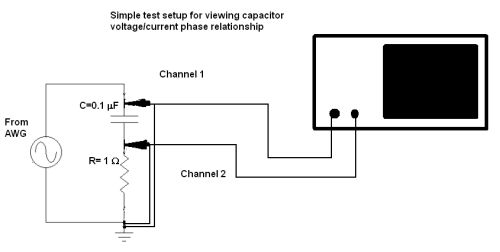
You can easily set up a circuit that shows the phase relationships between capacitor current and voltage. With the simple circuit diagrammed here, set the AFG or AWG to about 10 kHz with signal amplitude below about 10 V. The idea is to use a low value for R so that, basically, the voltage across R to ground represents capacitor current. It is best to trigger the scope from channel one which will be a cleaner waveform. Most scopes these days have cursor softkeys that will allow an exact measurement of phase difference between the two sinewaves.
You can also represent the phase shift in terms of a Lissajous pattern. Setting the horizontal mode to XY and leaving channel two to operate as before should generate an almost perfect circle, with a few adjustments to the V/div controls. The circle won’t be exactly perfect because of the finite resistance R adds to the circuit.


Leave a Reply
You must be logged in to post a comment.