Most engineers are familiar with the observation named after Gordon Moore, the co-founder of Fairchild Semiconductor and Intel, who in 1965 posited that the number of components on integrated circuits had doubled annually and projected this rate of growth would continue for at least another decade. In 1975, looking forward to the next decade, he revised the forecast to doubling every two years. His prediction has held since 1975 (though the rate has slowed recently) and has since become known as a “law.”
A less well-known “law” is Edholm’s law which asserts that the bandwidth of a telecommunication network doubles every 18 months. The success rate of this law has also been valid since the 1970s. More specifically, Phil Edholm of Nortel Networks observed that the three categories of telecommunication–wireless (mobile), nomadic (wireless without mobility) and wired networks–are in lockstep and gradually are converging. Edholm’s law also holds that data rates for these telecommunications categories increase on similar exponential curves, with the slower rates trailing the faster ones by a predictable time lag.
It is interesting to review some of the main factors that have allowed bandwidth and data rates to double every 18 months. Observers claim the most important factors have been the development of the metal oxide semiconductor field-effect transistor (MOSFET), the development of laser light wave systems, information theory, as enunciated by Claude Shannon at Bell Labs in 1948.
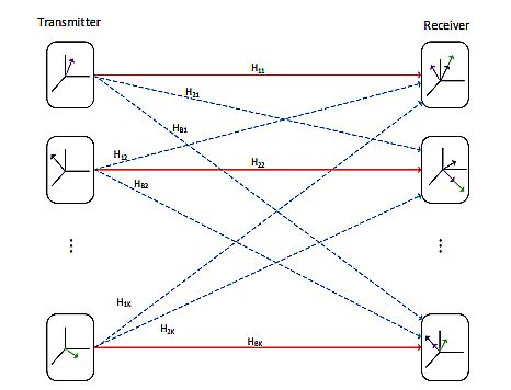
Most engineers are unlikely to have run into interference alignment in their work, but some have probably used a technology that makes use of some Interference alignment concepts: MIMO, or multiple-input and multiple-output methods for multiplying the capacity of a radio link using multiple transmission and receiving antennas to exploit multipath propagation.
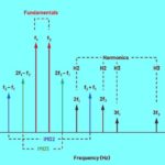
Interference alignment exploits the availability of what mathematically are called multiple signaling dimensions. In real life, the signaling dimensions can arise from use of either multiple antennas, time slots or frequency blocks. The transmitters linearly encode their signals over these multiple signaling dimensions such that the resulting interference signal observed at each receiver lies in a lower dimensional subspace (as when a signal is received from a subset of MIMO antennas) and is orthogonal to the one spanned by the signal of interest at each receiver. (At orthogonal frequencies, the individual peaks of frequencies of interest all line up with the nulls of the other frequencies.) This overlap of spectral energy does not interfere with the system’s ability to recover the original signal. All in all, interference alignment showed that theoretical limits on communication channel capacity could be orders of magnitudes higher than were previously thought possible, especially for large networks.
That brings us to MIMO. The technique can be sub-divided into three main categories: precoding, spatial multiplexing (SM), and diversity coding. Precoding occurs at the transmitter. In (single-stream) beamforming, the same signal is emitted from each of the transmit antennas with a phase and gain-weighting scheme that maximizes the signal power at the receiver input. Beamforming boosts the received signal gain by making signals emitted from different antennas add up constructively. (A point to note is that you must know a lot about the path between the transmitter and receiver to truly optimize the phase and gain weighting this way.) It also reduces the multipath fading effect. In line-of-sight propagation, beamforming produces a well-defined directional pattern. However, cellular networks are mainly characterized by multipath propagation. When the receiver has multiple antennas, the transmit beamforming cannot simultaneously maximize the signal level at all of them. Here precoding with multiple streams is often beneficial.
In spatial multiplexing, a high-rate signal is split into multiple lower-rate streams, and each stream is transmitted from a different transmit antenna in the same frequency channel. If these signals arrive at the receiver antenna array with enough spacing and the receiver has accurate CSI (channel state information; in other words, it knows the combined effect of scattering, fading, and power decay with distance), it can separate these streams into (almost) parallel channels. Spatial multiplexing is a way to boost channel capacity at higher signal-to-noise ratios (SNR). The maximum number of spatial streams is limited by the lesser of the number of antennas at the transmitter or receiver. Spatial multiplexing can also be used for simultaneous transmission to multiple receivers, known as space-division multiple access or multi-user MIMO. Here, the transmitted signal must take into consideration the CSI factors.
Diversity coding techniques are used when the transmitter doesn’t know anything about the CSI it will encounter. In diversity methods, a single stream (unlike multiple streams in spatial multiplexing) is transmitted, but the signal is coded using what’s called space-time coding. The transmitted signals are set up to be orthogonal to each other. Diversity coding exploits the independent fading in the multiple antenna links to enhance signal diversity. Because there is no CSI, there is no beamforming or array gain from diversity coding. Diversity coding can be combined with spatial multiplexing when the receiver knows something about the channel properties.


Leave a Reply
You must be logged in to post a comment.