Why does the Fourier transform provide apparently inaccurate results, and what can I do about it? part 2

A bare-bones implementation of the Fast Fourier Transform helps illuminate how to extract frequency information from input data samples.

In part 1 of this series, we reviewed the discrete Fourier transform (DFT) and manually calculated one DFT shown in Table 1.

Table 1. Manual DFT results

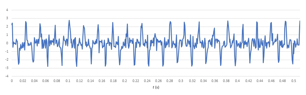
The point of the DFT is to extract frequency content from an input function of time, and as you pointed out, frequency information is not apparent in our result. We concluded part 1 by beginning to set up an Excel worksheet to perform a Fast Fourier Transform (FFT) on the time-domain signal in Figure 1.Didn’t you mention that the preferred tool for running the DFT on a computer would be engineering software such as MATLAB or LabVIEW?
Right, but the bare-bones nature of the Excel implementation makes it useful for examining some details that take place behind the scenes in more elegant solutions.

We defined six worksheet column headings last time. What goes into each column?

Figure 2 provides the details; just follow the nine steps listed in red. Note that in column B, we enter the times for our data samples, thereby mapping sample n to time t. Then we insert our 512 sample data points into column C, which serves as the DFT input.

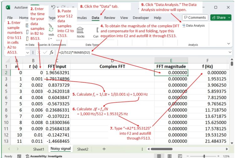
We reserve column D for the FFT complex output. For column E, we calculate the magnitude of column D using the Excel IMABS() function, which returns the absolute value of a complex number. In addition, to normalize the FFT magnitude so that a frequency pulse with a magnitude of 1 corresponds to a sinusoid with a peak value of 1, we multiply the column E values by 2/N.
Now we can develop our frequency scale. Note that the sampling interval is

Δt = t_n– t_n-1

or 1 ms in this example, and Δt appears explicitly in cell B3. In step 5, we calculate the sampling frequency f_S, and in step 6, we calculate Δf, or 1.95 in this case. Beginning with 0 in F2, successive cells in F will increase by Δt until we reach cell F513. A convenient way to fill F2 through F513 is simply to multiply n by 1.95 (step 7).

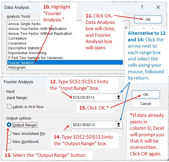
Continue with steps 8 and 9, and Data Analysis box appears (Figure 3 top). Continue with steps 10 and 11, which will open the Fourier Analysis box (Figure 3, bottom), where you can complete initiation of the FFT using steps 12 through 15.

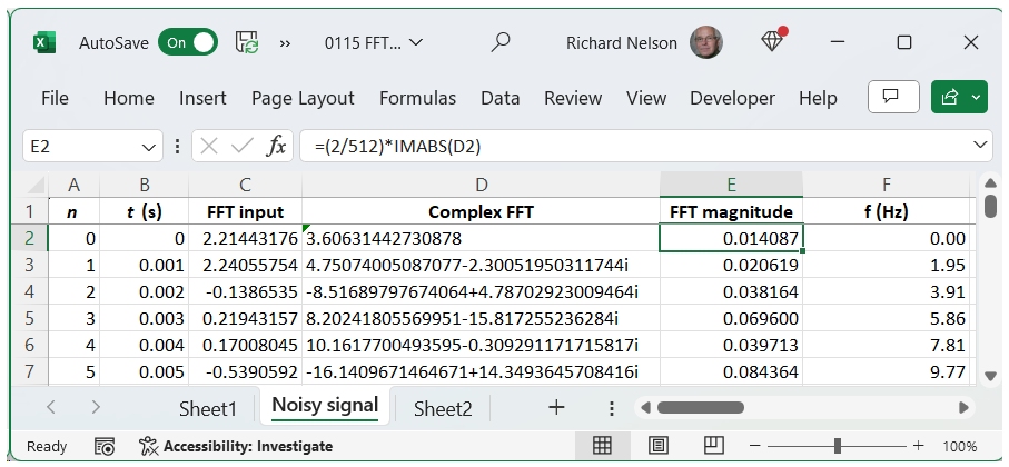
After a few seconds, Excel will write the complex FFT into column D, and the FFT magnitude will appear in column E (Figure 4).

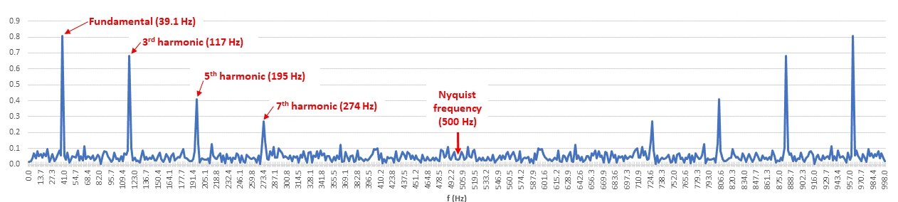
Now we can plot the FFT magnitude in column E vs. frequency in column F (Figure 5). The FFT shows noise throughout the frequency range but with distinct peaks at a 39.1-Hz fundamental frequency plus the third, fifth, and seventh harmonics. Note that the FFT creates a mirror image of these pulses above the 500-Hz Nyquist, or folding, frequency. These aliases may be discarded, and in subsequent charts I will only include frequencies up to the Nyquist frequency.

Interesting. How much confidence can we have in these results?

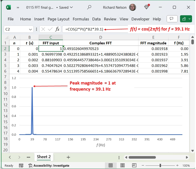
To answer such questions, it can be useful to apply a clean signal to the DFT and then alter it in various known ways to determine how the DFT responds. Let’s take a quick look. In Figure 6, in place of the Figure 1 waveform data I have substituted a clean cosine wave of the Figure 5 signal’s 39.1-Hz fundamental frequency. As expected, the FFT produces a pulse of magnitude 1 at 39.1 Hz.

Now, let’s tweak our cosine wave—we won’t add any interference but just reduce the frequency by about 2.5% to 38.12 Hz. Now, take a look at the FFT in Figure 7.

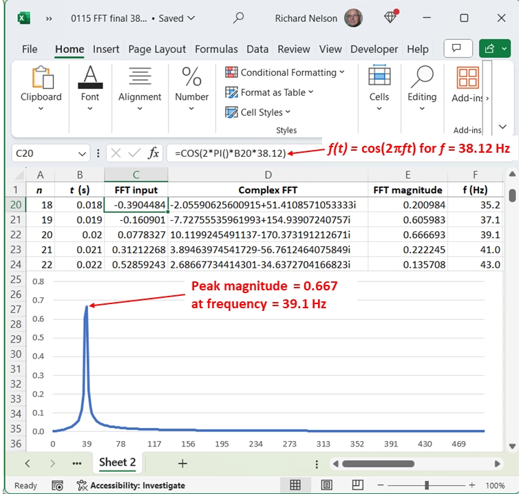
The peak frequency still appears at 39.1 Hz, but its magnitude is reduced to 0.667, What happened? (Hint: Figure 7 contains a small clue.) We’ll take a closer look in part 3.