Why does the Fourier transform provide apparently inaccurate results, and what can I do about it? part 3

Windowing functions account for mismatches between an input signal and FFT sample size.

We concluded part 2 of this series with a look at fast Fourier transforms (FFTs) of 39.1-Hz and 38.12-Hz cosine waves, with our sample size N = 512 and our sample interval Δt = 1 ms (Figure 1).

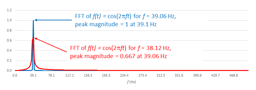
Shouldn’t the amplitudes of both traces be 1?
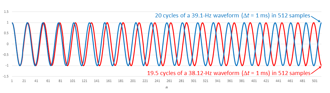
Yes. Figure 2 shows why they’re not: 20 cycles of the 39.1-Hz waveform fit into our sample space, but only 19.5 cycles of the 38.12-Hz waveform fit.

Why is that a problem?

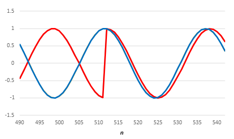
The FFT assumes that our finite data set extends infinitely. Figure 3 shows what happens about the 512th sample. The red waveform exhibits a discontinuity, or, within the limits of our sampling, a very steep ramp, which represents energy at frequencies beyond our Nyquist limit. This effect is called spectral leakage.

Can we adjust our sample size to compensate?
That’s not convenient since generally we are acquiring unknown signals. Also, Excel’s FFT algorithm requires that N be a power of 2, so we can’t just add a few extra samples to give the red wave time to catch up.

What’s the solution?

We apply windowing functions, which provide near-unity gain near the center of our sample set and increasing levels of attenuation near the beginning and end. Many windowing functions find use. (See Understanding FFTs and Windowing from NI for more on what windows to apply for specific situations.) Figure 4 plots amplitude vs. sample n for two common ones: the Hamming window (as described in a 1976 Naval Undersea Center paper) and the flat top (a normalized version of a flat top described in a 1987 Brüel & Kjær Technical Review).

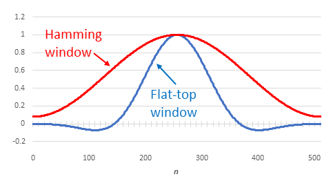
Figure 5 shows the Hamming window applied to our 38.12-Hz waveform, where the FFT peak amplitude is 0.448.

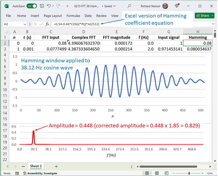
That’s even lower than 0.667 of Figure 1.
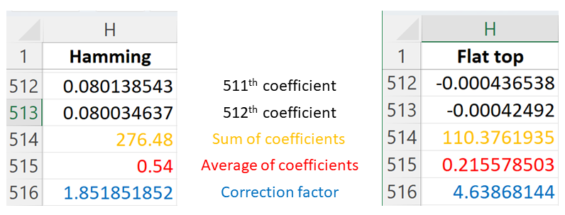
Right, because the overall effect of a window is attenuation. We need a correction factor, which we can obtain by scrolling down to the bottom of column H and computing the inverse of the average of the Hamming coefficients (Figure 6 left): 1.85 here, so our corrected amplitude is 0.829.

That’s still short of 1.
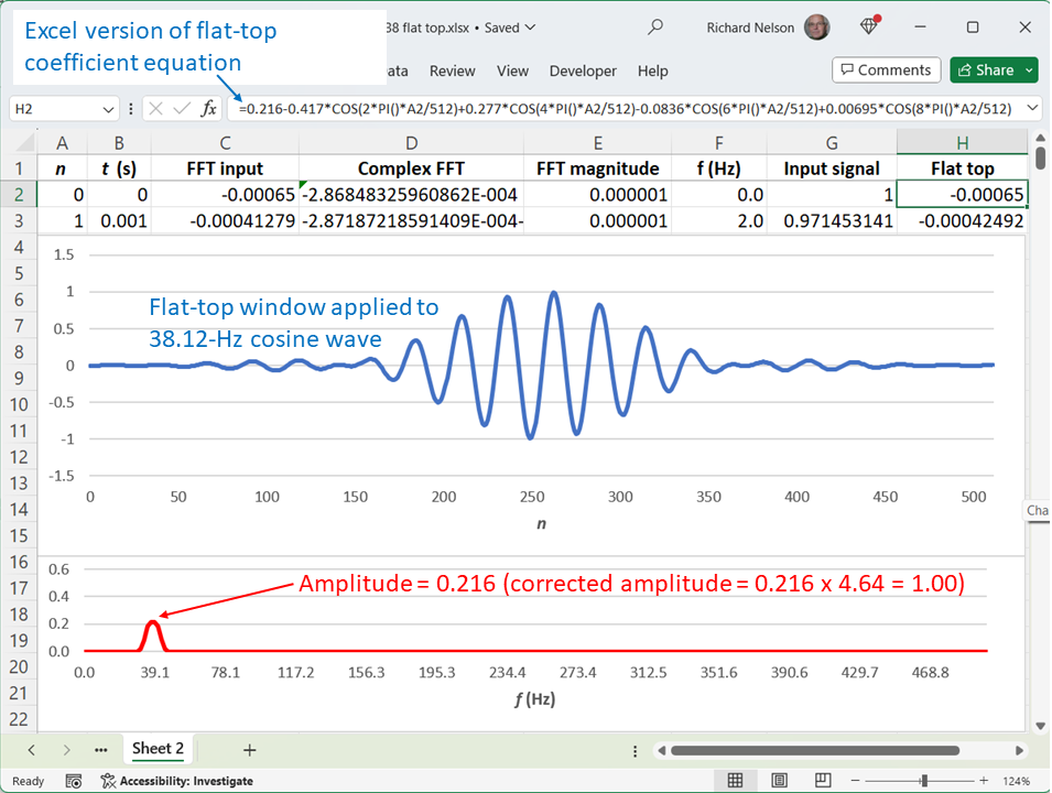
Let’s try the flat top (Figure 7). Sure enough, the flat-top window with the appropriate correction factor (Figure 6, right) provides good amplitude accuracy.

Note that these correction factors apply only to amplitude.
Window functions also have energy-correction factors, which differ numerically from amplitude correction factors (as described in an article from Siemens).

Why is the peak not 38.12 Hz?

If you look back at Figure 7 in part 2, you’ll see that 39.1 Hz is the closest “frequency bucket” to 38.12 Hz, an indication that 38.12 Hz isn’t going to be an ideal fit for our sample space.

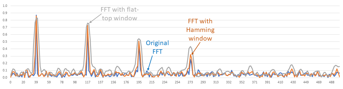
In part 2, you presented the FFT with a 39.1-Hz fundamental plus third, fifth, and seventh harmonics. Does windowing affect that result?

Good question and the answer is not much. Figure 8 shows the unwindowed and windowed FFTs. The FFT does indeed provide an unexpected result, but spectral leakage is not the issue, and windowing is not the fix.

What is the issue?

Throughout this series, we have focused on amplitude, but an earlier series on phase noise (see part 1 and part 2) inspired this look at the FFT. In the final part of this series (part 4), we’ll return to the phase-noise topic and its applicability to the Figure 8 signal, and we’ll show how to use the FFT to make phase measurements.