A mixer can upconvert and downconvert a modulated signal with no loss of baseband information. Part 1 of this series described intermodulation resulting from the combining of two or more sinusoidal signals through a nonlinear device such as the mixer in Figure 1. The mixer’s output is the product of its two inputs, and its […]
What is intermodulation, and is it good or bad? Part 1
Sinusoidal inputs applied to a nonlinear system produce an output containing different frequencies, and the results can be good, bad, or ugly. According to the dictionary definition, intermodulation is “the production in an electrical device of currents having frequencies equal to the sums and differences of frequencies supplied to the device.” In the literature of […]
Why does the Fourier transform provide apparently inaccurate results, and what can I do about it? Part 4
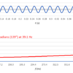
The FFT can measure phase angle, but what appears to be a meaningful result might just be the arctangent of a ratio of rounding errors. Throughout this series, we reviewed the fast Fourier transform (FFT) as implemented in Microsoft Excel and investigated windowing functions. In this final part, we’ll cover phase measurements, but first, let’s […]
Why does the Fourier transform provide apparently inaccurate results, and what can I do about it? part 3
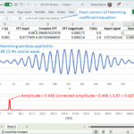
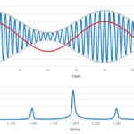
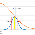
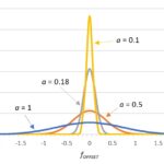
Windowing functions account for mismatches between an input signal and FFT sample size. We concluded part 2 of this series with a look at fast Fourier transforms (FFTs) of 39.1-Hz and 38.12-Hz cosine waves, with our sample size N = 512 and our sample interval Δt = 1 ms (Figure 1). Shouldn’t the amplitudes of […]
Why does the Fourier transform provide apparently inaccurate results, and what can I do about it? part 2

A bare-bones implementation of the Fast Fourier Transform helps illuminate how to extract frequency information from input data samples. In part 1 of this series, we reviewed the discrete Fourier transform (DFT) and manually calculated one DFT shown in Table 1. Table 1. Manual DFT results DFT input Complex DFT |DFT| 3 12 + j0 […]
Why does the Fourier Transform provide apparently inaccurate results, and what can I do about it? part 1

This multipart series will review the discrete Fourier Transform and describe how to avoid common problems when transitioning from the time to frequency domain. A recent post on phase noise discussed expressing a function of time as a function of frequency. The Fourier Transform is the well-known road from the time domain to the frequency […]
What is phase noise and how can I measure it? part 2
Phase noise requires more than one instrument unless you use a phase-noise analyzer.
What is phase noise, and how can I measure it? part 1
Phase noise is an artifact of a nonideal oscillator and is best investigated in the frequency domain. Phase noise accompanies the generation of any real-world sinusoidal signal. You can think of it as the analog equivalent of digital jitter, which we covered in an earlier series (read part 1 and part 2). Recall that jitter […]
How to test the automotive SENT protocol
Oscilloscopes and dedicated software can help analyze SENT data. In “What is the automotive SENT protocol?” we looked at the Single Edge Nibble Transmission (SENT) protocol, as defined in accordance with the Society of Automotive Engineers (SAE) J2716 standard. We reviewed the SENT message frame, which includes a synchronization/calibration pulse followed by a status nibble, […]
How do I choose an electric motor, and how do I test it? part 4
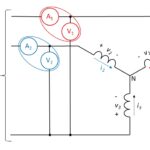
You indeed can measure three-phase power in a motor with just two wattmeters. Part 3 of this FAQ concluded with a simplified diagram showing a test setup that included a programmable power supply, a motor under test, a mechanical load, a power analyzer, and host computer. The programmable power supply could simulate the AC line […]
