Differences between stand-alone and scope-based spectrum analyzers

Most oscilloscope manufacturers also offer an extensive line of spectrum analyzers. There are similarities as well as differences between these two distinct instruments. The oscilloscope is optimized to display signals in the time domain, its default mode. Additionally, pressing Math>FFT, the same signal appears in the frequency domain. In the Tektronix MDO (mixed domain oscilloscope), the same signal can be plotted not in split-screen format as in Lissajous patterns, but against a common set of Cartesian coordinates.

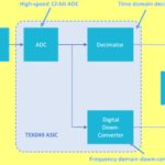
Scopes in the spectrum-analyzer mode process signals differently than some stand-alone spectrum analyzers (SAs). Digital scopes basically digitize their input, then apply a mathematical fast Fourier transform (FFT) function to calculate a frequency content and amplitude.

One thing that complicates the comparison is that some spectrum analyzers do exactly the same thing — digitize the waveform and calculate an FFT. But this approach has some downside, including a reputation for more harmonic noise when there is signal energy outside the expected measurement range. That is why there is room for true SAs, which work differently. They measure the amplitude at each frequency the signal contains using dual or triple-down-conversion swept scanning. They needn’t do a calculation to generate a display. In addition, true SAs generally digitize signals via DACs of at least 16-bits whereas scopes may more typically employ eight and 12-bit DACs. The longer digital word length provides a higher dynamic range.

That said, it is also possible to find scopes combined with swept SAs. But these tend to be pricey instruments.

With these differences in mind, we’ll cover a few basics. In the frequency domain, the spectrum analyzer plots amplitude on the Y-axis, but now the Y value is power rather than voltage. The X-axis represents frequency rather than time. Time-domain and frequency-domain displays of the same signal contain the exact same information, but they have an altogether different look. In the time domain, low-level harmonics and noise appear as a slight thickening of the trace, hardly noticeable and difficult to identify. In the frequency domain, they are prominent spikes or an elevated noise floor.

A signal in the time domain can be transformed into a signal in the frequency domain by means of calculations known as Fourier analysis, and the reverse transformation can be accomplished by means of Fourier synthesis. This transformation back and forth can take place indefinitely with no loss of information, subject only to losses in the instrumentation.

The Fourier transform is a complex and lengthy mathematical process, vastly simplified in the Fast Fourier Transform (FFT), which was made accessible in the 1960s. It can be performed instantly in modern digital storage oscilloscopes by pressing a couple of buttons.

Each of the complementary domains reveals different aspects of the waveforms at the oscilloscope inputs. In the time domain, we see the waveform’s shape, and this provides an intuitive look at its unique periodicity. But it is the frequency domain that reveals the waveform’s spectral distribution – the amount of energy it contains at discrete frequencies. Many advanced engineers glance quickly at the time domain display before turning to the frequency domain to see what is really going on.

A swept-tuned SA, the type generally associated with stand-alone SAs, consists of a voltage-controlled oscillator, which in classic heterodyne fashion down-converts the desired range of frequencies subject to the bandwidth of the instrument. The voltage that controls the oscillator and hence the frequency of the signal that is displayed at any given moment moves across the frequency range under investigation, displaying amplitude peaks where harmonics exist. A bandpass filter determines the frequency range. A smaller range has the advantage of providing greater spectral resolution, meeting the needs of some applications. It is helpful for distinguishing adjacent frequency components, although at the cost of reduced bandwidth. A relevant equation is:
S_T = kf/R_BW, where S_T is sweep time in seconds, k is a proportionality constant, f is the frequency range in Hertz, and R_BW is resolution bandwidth in Hertz.

In an FFT-based spectrum analyzer, the frequency resolution is Δv = 1/T.
This is the inverse of the time T during which the waveform is measured as subject to Fourier analysis. The input signal is sampled at a rate sufficient to comply with Nyquist requirements. FFT-based spectrum analyzers have limited range due to ADC and processing power for the Fourier transform capabilities.

There is a third type of SA known as a real-time spectrum analyzer. It is not prone to these limits up to the maximum span, known as the real-time bandwidth. Using FFT processing, it samples the incoming RF spectrum in the time domain and converts that data to the frequency domain by means of FFT processing. This type of spectral analysis still has gaps due to time requirements for processing. The gaps are filled in, however, by means of overlapping near-simultaneous acquisitions. Thus, real-time spectrum analyzers provide a more complete and detailed image in the frequency domain of the signal of interest.

In all SAs, pressing the RF button, the user is confronted with Center Frequency, Span, Start and Stop. (Don’t be confused with R to Center. That just has to do with placing a reference marker.) The Frequency and Span values have to be set properly to get a good display.

To begin, unless you plan to try random values, you have to know the frequency of the signal at the input. If you are looking at the utility power supply, single-phase or three-phase, you know that it is 60 Hz, or in some areas 50 Hz. If you are looking at a waveform from the internal AFG, there are certain default frequencies, or the frequency may be user-determined by pressing Waveform Settings. You can check the frequency by looking at the horizontal AFG bar at the bottom left of the screen, just above the horizontal menu bar. For most waveforms, the default is 100.00 kHz. Some waveforms, such as dc, Noise and Exponential Rise and Decay have no stated frequency because they are nonperiodic.

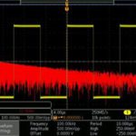
If you do not know the frequency, go to Measure>DVM>Frequency, and it will be displayed. Then, with the BNC cable feeding the AFG signal to the RF input, press the Freq/Span button, which opens the vertical Frequency and Span menu on the right. Most people like to bring the fundamental to the center of the screen. To do this, set the Center Frequency to 100.00 kHz or other appropriate signal frequency. Notice that with the sine wave, all the power is in the fundamental with no harmonics.

But not so fast! The default span is way too high to see harmonics anyway. To display harmonics or verify the absence of them we’ll want to look at a square wave. Press AFG>Waveform and scroll down to Square Wave. Still no harmonics except for a slight perturbation at the base of the fundamental. Recall that the highest amplitude harmonic other than the fundamental, which is actually known as the first harmonic, is the second harmonic. Then the harmonics fall in amplitude as they get farther away in frequency from the fundamental, eventually disappearing below the noise floor.

So, going back to Freq/Span, try 10, 20 and 30 MHz in the Span field. There are two things to notice here. When you set Span, Start and Stop adjust themselves. If you set Start and Stop, Span adjusts itself. Therefore, do not fill in more fields than necessary. Secondly, a smaller span allows you to see the harmonics at greater resolution, while a larger span allows you to see how they diminish in a logarithmic fashion. Press Menu Off to get a better view. Above a 30 MHz span, the individual harmonics are difficult to count.

Going back to Sine, we can view in these more revealing frequency and span settings that there are indeed no harmonics. You can see that the fundamental extends to the noise floor, which is the result of thermal noise in the instrument’s circuitry. The fact is that all conductors, including electronic components, exhibit thermal noise unless they happen to be at absolute zero degrees Kelvin.

Any conductor will have a tiny but measurable voltage across it, and if the ends are shunted together, a minute current flows. The noise floor is what you are seeing in that fluctuating irregular roughly horizontal line in the lower part of the screen. It is a barrier below which no signal can be measured or displayed. It should be regarded not as a defect, but rather as evidence of the great sensitivity of this auto-ranging instrument. That said, instrumentation engineers are always trying to lower the noise floor so fainter signals can be displayed.

If you want to see something interesting, press the BW button below RF. You see the noise floor as it generally appears. The resolution bandwidth (R_BW) is on Auto at its default 30.0 kHz value. Turning Multipurpose Knob a clockwise, RBW Mode moves to manual and as the bandwidth decreases, the resolution rises. (They are always inversely related.) If you bring it up to its limit, 1.50 MHz, the noise floor has quite a different look. Of course, the signal is no different. The change is in how it displays.