Working with waveforms in mixed-domain oscilloscopes

Waveform generators generally contain a library of common waveforms, which can be individually accessed and displayed by running a BNC cable to an active analog channel input in an oscilloscope. Most oscilloscopes have, available as an option, an internal arbitrary function generator (AFG), which permits the user to create an endless variety of waveforms and display and save them to internal memory or to an external medium. These internal AFGs also have a selection of pre-made waveforms, although not as extensive as in the stand-alone bench-type waveform generators.

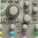
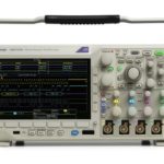
The Tektronix MDO3000 Series oscilloscope’s internal AFG has a library of 13 permanent waveforms. To access them, run a BNC cable from AFG Out on the back panel to an active analog channel input. Press AFG. The default selection is sine wave, and it immediately appears in the display. The AFG bar at the bottom left of the display shows the default frequency, 100.00 kHz, and the default amplitude, 500 mV peak-to-peak. The user can change these values. Press the soft key associated with Waveform Settings. The vertical Waveform Settings menu appears at the right of the display. Multipurpose Knob a or the keypad can change the frequency. Its reciprocal, period, automatically changes. Similarly, amplitude can be adjusted. You may have to press Autoset to see the new waveform in the display. To go back to the default values, use Multipurpose Knob a or the keyboard, or press Default Setup and turn back on the AFG.

Pressing the soft key associated with waveform, you will see in the vertical menu at the left that any of the 13 available waveforms can be selected. But first, going back to sine, we’ll see why this is called a mixed domain oscilloscope (MDO), not to be confused with a mixed signal oscilloscope (MSO), which is a different instrument altogether.

With the sine wave displayed, press Menu Off to get a better view of the waveform. Then, press the red Math button just to the right of the display. In the horizontal Math menu that appears below the display, press the soft key associated with FFT. Again, press Menu Off to declutter the display.

What we see now is the original sine wave displayed in the time domain, and the same signal with Fast Fourier Transform applied to create the frequency domain display. In an ideal sine wave all the power is at the fundamental frequency, which is technically known as the first harmonic. Thus, in the frequency domain trace you see a single prominent spike at the left of the display. The irregular, rapidly fluctuating roughly horizontal line represents the noise floor of the oscilloscope. This is not a flaw or fault in the instrument. It is a consequence of thermal energy (random particle motion) that appears as a very small voltage across any conductor or device when it is not connected to a load. If the leads are shunted, there is actually current flow, and this is what you see in the noise floor. Portions of the signal that have less amplitude than the noise floor cannot be displayed. This same noise floor is less prominent in the time domain display, but it appears as a slight thickening of the trace, which can be dramatically mitigated by means of bandwidth limiting or signal averaging.

In the time domain, values in the X-axis represent time, while in the frequency domain they correspond to frequencies in the displayed spectrum. In both domains, the Y-axis represents amplitude. In the time domain, amplitude is measured in volts, while in the frequency domain amplitude is expressed in power. The frequency domain instrument, either an oscilloscope or a spectrum analyzer, can be configured by the user to show this power on either a logarithmic scale, the default, or a linear scale.

We can keep the oscilloscope in the FFT mode while scrolling through some other AFG waveforms. To do so, press AFG once more. This brings up the horizontal AFG menu. Press the soft key associated with waveforms, bringing up the vertical waveform menu at the left. Use Multipurpose Knob a to scroll down to the next waveform on the agenda, Square Wave.

Then press Menu Off to get the waveform menu out of the way so we can view this interesting mixed-domain display. In looking at the time-domain display, we are seeing a graph of the signal amplitude in volts, plotted against the passage of time. The signal is comprised of two voltage levels and because it is not offset, they are equal in magnitude but opposite in polarity. The transitions appear to be instantaneous but actually there are brief rise and fall times, which become increasingly apparent as we raise the frequency.

The defining characteristic of a square wave is its 50% duty cycle. The duration of the high and low levels are equal, and that’s what distinguishes the square wave from the pulse wave, of which it is a special case.

The square wave, as generated in an oscillator, is widely used as a clock signal for computer and oscilloscope circuits, for example, to facilitate sampling in an ADC. Wherever there are digital signals that have to be handled in a way that is not asynchronous, there is a clock outputting a square wave.

Because the fast rise and fall times are high-frequency components of the square wave, the square wave has a significant harmonic content. You may be able to predict this by looking at the time domain representation, but in the frequency domain, it is more readily apparent. Rather than the single strong spike at the fundamental as in the sine wave, there are many smaller spikes that gradually diminish in amplitude as they get farther away in frequency from the fundamental.

Pressing AFG>Waveform once more, we’ll scroll down to Pulse. This is similar to the square wave except that the duty cycle is not constrained to 50%. Here again, due to the fast rise and fall times, there is a great amount of harmonic power distributed in a manner that is similar to the square wave. Because the rise and fall times for this particular pulse happen close together in time with a relatively long interval during which the amplitude remains at the low level, in the frequency domain the spikes are discrete, eventually as always sinking below the noise floor.

Skipping down to Noise, this signal has a totally different appearance from those we have seen, both in the time domain and in the frequency domain. That is because in amplitude it is random with respect to time and in frequency it is non-periodic. As a product of random particle activity, the frequency is unbounded. The apparent high limit is a consequence of the measuring instrument’s finite bandwidth. If you press the analog channel button followed by Bandwidth, the vertical Bandwidth menu appears. It would seem that we have lost the frequency domain display, but it is still there, mostly hidden behind the time domain display. You can tell because now and then a red frequency domain peak appears below the time domain display trace. Cutting the bandwidth to 20 MHz causes the noise waveform in the time domain to further contract, and a larger part of the frequency domain signal comes into view. Noise is a very broad-spectrum phenomenon, and that is why bandwidth reduction causes the waveform amplitude to contract dramatically.

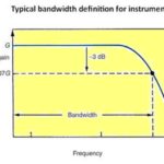
(Before proceeding, it is necessary to set Bandwidth back to Full.) Pressing

AFG once more, scroll down to Sin(X)/x. This is an interesting “waveform,” as the electronic engineer would say, while the mathematician would say “function” – they are really the same.

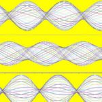
If you look at Sin(X)/x in the time domain, you will see that it is made up of closely-spaced spikes in regularly occurring clusters, with exponentially diminishing peaks that level out to a minimum value, slowly at first, then exponentially rising to comprise another cluster of high spikes.

In the frequency domain, Sin(X)/x is 1 as x approaches 0. It is a practical matter as well. Sin(X)/x provides a ringing pulse that is useful for looking at circuits with inductance. A sharp single pulse will have ringing in an inductive circuit where the higher frequence components are cut off. This function simulates that behavior.