Part 3 of a series on using near-field probes for detecting EMI sources shows you how to set up a spectrum analyzer and how to detect emissions problems.
Now that we’ve discussed the theory of measuring near-field emissions (Part 1) and how to use near-field probes (Part 2) to make the measurements let’s discuss how to interpret the results.
Knowing how to interpret what you see in the spectrum analyzer will help determine where to mitigate EMI issues. This will require a little explanation of narrowband versus broadband emissions.
The definition of whether a signal is narrowband or broadband as measured using a spectrum analyzer, depends entirely on the receiver bandwidth (resolution bandwidth, or RBW). For commercial measurements, the test standards define the RBW.
For example, when measuring conducted emissions from 150 kHz to 30 MHz, the RBW is specified as 9 kHz according to most commercial EMC standards. For frequencies between 30 MHz and 1000 MHz, the RBW is specified as 120 kHz. This was originally defined as the typical broadcast radio (AM and FM) receiver bandwidths.
Some low-end “affordable” spectrum analyzers may not be able to set these RBW values. Fortunately, setting RBW to 10 kHz and 100 kHz, respectively, is close enough for troubleshooting purposes. Figure 1 compares narrowband and broadband signals relative to a spectrum analyzer’s RBW.
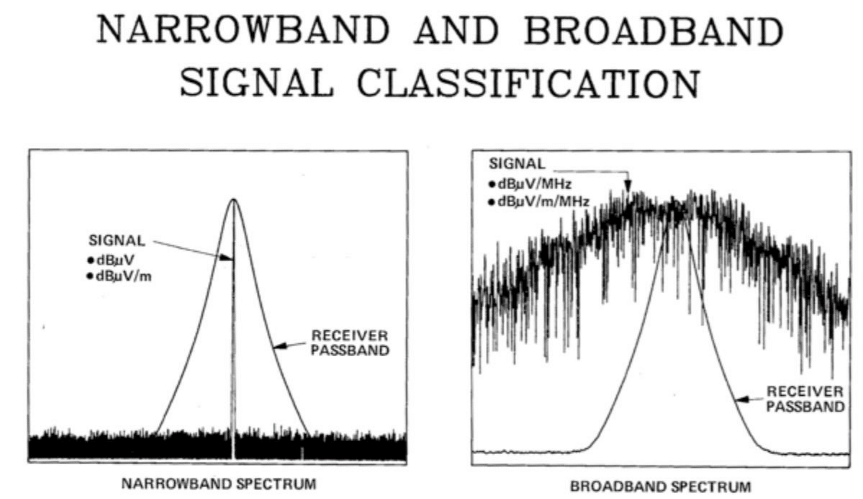
Narrowband includes continuous wave (CW) or modulated CW signals. Examples might include clock harmonics from digital devices, co-channel transmissions, adjacent-channel transmissions, intermodulation products, and so on. On a spectrum analyzer, narrowband signals appear as narrow vertical lines or slightly wider modulated vertical peaks associated with specific frequencies.
Broadband primarily includes switch-mode power supply harmonics, digital bus signals, arcing in overhead power lines (power line noise), wireless digitally-modulated systems (such as Wi-Fi or Bluetooth) or digital television. On a spectrum analyzer, this would appear to be broad ranges of signals or an increase in the noise floor. Digital bus noise or switch-mode power supplies are the most common broadband signal sources.
Note that by reducing the RBW down to 1 kHz or so, you can start resolving the harmonics from DC-DC converters or other switching power supplies. You’ll see that the harmonic signals are narrowband signals. This illustrates that a series of harmonic signals can be both narrowband and broadband. It all depends on the RBW setting. To avoid confusion, select RBW settings according to the EMC standard to which you’re testing.
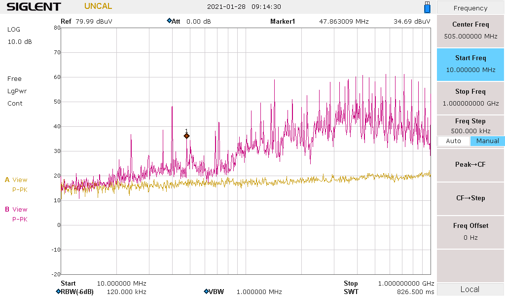
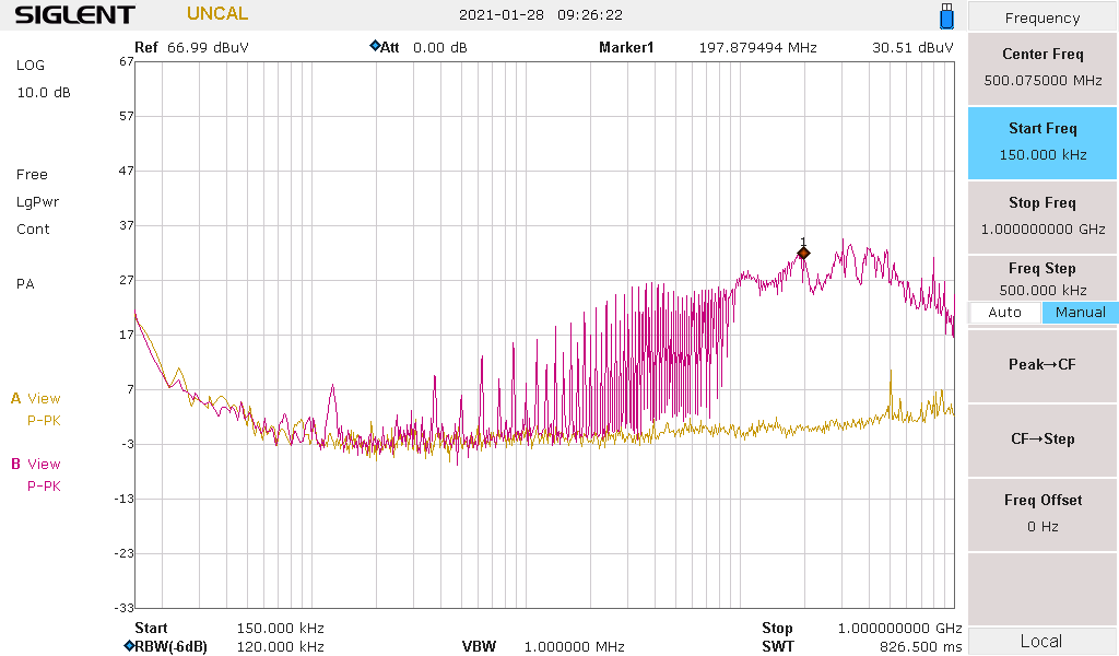
Figures 2 to 8 demonstrate examples of common harmonic profiles for different on-board sources that I often see in practice. Note that it’s common to have a combination of narrowband emissions riding along on top of a broadband emission. In all figures, the yellow trace represents the measurement noise floor.
Figure 2 shows a frequency sweep from 10 MHz to 1000 MHz. The narrowband 48 MHz clock includes spikes every 48 MHz.
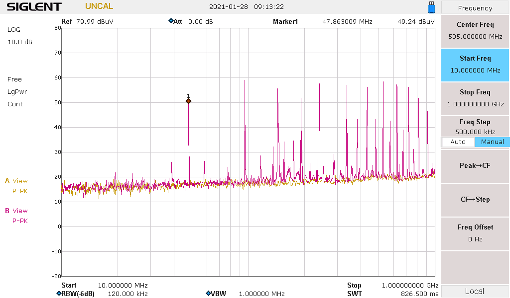
Figure 3 shows another sweep from 10 MHz to 1000 MHz. This time, the sweep shows a broadband noise signal with narrowband spikes.
The sweep from 150 kHz to 1 GHz in Figure 4 displays typical broadband DC-DC converter noise. This self-generated EMI can couple to sensitive wireless receivers and cause lack of sensitivity.
In Figure 5, the display shows a typical spread-spectrum clock signal, which is typically classified as narrowband. You can, however, see the energy spread, the result of modulating the CW clock with either dithering or direct sequence spread spectrum. The result: an effective lowering of the narrowband amplitude, which often makes meeting emission limits easier. This is commonly used on computers where the clock skew is less important.
The sweep in Figure 6 shows a structural resonance caused by an attached 2-m long cable to the PC board under test. The resonant frequency is approximately 90 MHz.

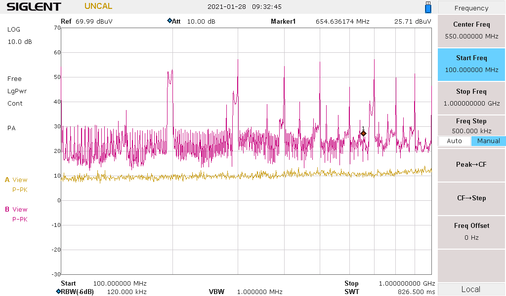
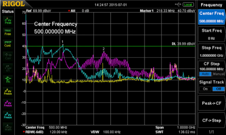
Switch-mode power converters commonly exhibit ringing on the switched waveform. This ringing can appear as broadband peaks, such as in Figure 7. Marker 1 highlights the 217 MHz ringing on a GaN converter running at 1 MHz. The first peak in the aqua trace (marker 1) is the primary 217 MHz ring frequency while the second peak (marker 2) on the violet trace is the second harmonic at 434 MHz.
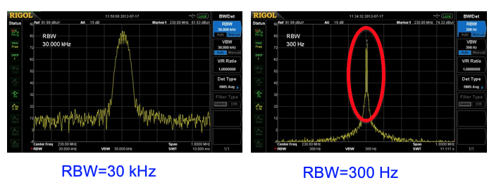
If you reduce the RBW sufficiently on a narrowband harmonic, you may observe a ripple effect at the top (left image in Figure 8). Reducing the RBW even further will likely reveal two harmonics at the same frequency, created by two different clock sources (right image)! This is a good reason to keep potential fixes in place until both sources are mitigated, otherwise, it might seem as if the first fix did not help.
Summary
Once we’ve identified and recorded the emission profile for each dominant energy source on the board, we’ll be turning our attention to some system-level measurements like attached cables and seams in shielded enclosures. Because power, I/O cables and enclosure seams are sometimes long enough to act like efficient antennas, we’ll learn how RF current probes can be used to characterize RF cable currents and use our near field probes to assess seam leakage in the next article.
References
Wyatt, Kenneth, Create Your Own EMC Troubleshooting Kit (Volume 1, 2nd Edition), Amazon, 2022
Wyatt, Kenneth, Workbench Troubleshooting EMC Emissions (Volume 2), Amazon, 2021


Leave a Reply
You must be logged in to post a comment.