How do you measure phase noise?

Phase noise is an artifact of a nonideal oscillator and is best investigated in the frequency domain.

Phase noise accompanies the generation of any real-world sinusoidal signal. You can think of it as the analog equivalent of digital jitter, which we covered in an earlier series (read part 1 and part 2). Recall that jitter results from deviations from the ideal positions of the rising and falling edges of square waves, and it can be quantified in the time domain as peak-to-peak or rms jitter measured in picoseconds or other time units.

How does phase noise differ from jitter?

By way of background, Figure 1 shows two ways of representing an ideal sine wave: the time-domain view (a) and the frequency-domain view (b).

Figure 1. A sine wave can be represented in the time domain (a) or frequency domain (b).

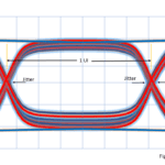
Obviously, real-world sine waves won’t look like the one in Figure 1. Figure 2 shows a more realistic example of sine-wave traces that might come from a real-world oscillator. The blue trace appears close to our ideal 1-GHz example. The red trace appears to maintain the same frequency but at a slight phase delay. The gray trace’s frequency has drifted high, while the yellow trace’s frequency has drifted low. All these variations contribute to phase noise.

Figure 2. Phase shifts and frequency drift contribute to phase noise.

I see the zero crossings near the 0.5-ns point all occur at different times. Can we measure the time differences to characterize phase noise?

We could make those measurements and get results in terms of picoseconds or even degrees or radians of phase shift. That approach works well for square-wave jitter. If a square wave has 10 ps of peak-to-peak jitter, you should sample your data more than 10 ps after one edge and more than 10 ps before the next edge. But for a sine wave, the exact positions of the zero crossings don’t usually lead to any direct insights that we can apply to our designs.

So, perhaps we need to look at the frequency domain.

Right. In Figure 1b, the vertical arrow at 1 GHz represents infinite energy in a pulse 0 Hz wide. The infinite energy arises because the Fourier transform that gets us from Figure 1a to Figure 1b assumes that our sine wave extends back in time to minus infinity and will continue to plus infinity. The value of 1 in Figure 1b represents the normalized value of the integral of the total area in the frequency domain from minus infinity to plus infinity. The Figure 1 performance is not attainable in real life.

What does the real-world frequency domain look like?

We can approximate the impulse response using the Dirac delta (δ) function, which is often expressed as follows:

Here, for our purposes, the independent variable f represents frequency and δ(f) represents power. Figure 3 shows what δ(f) looks like for various values of a, where 0 on the x axis indicates the center, or carrier, frequency (not 0 Hz), and the nonzero x-axis values represent offsets from the center frequency.

Figure 3. Different values for the variable result in different δ (f) curves.

OK, I see that our goal is to keep the response as narrow as possible around the center frequency at 0. Is that right?

Right. Keep in mind that the sidebands — the regions to the left and right of the center frequency, could contain useful message information if the carrier is modulated. But if you are looking at the output of a fixed-frequency oscillator, then the sidebands represent only phase noise. Note that in Figure 4, the gray signal, with lots of phase noise, swamps the red signal, whereas the blue signal, with much less phase noise, and the red signal can peacefully coexist.

Figure 4. The gray signal swamps the red signal, but the red and blue signals can coexist.

How do we put a number on phase noise?
Phase noise is typically specified in decibels relative to the carrier (dBc) per hertz at an offset from the carrier, or center, frequency. Figure 5 shows the process, with a power measurement taken over a 1-Hz band at a distance f_OFFSET from the carrier. Vendors often specify phase noise for a range of offsets. You might, for example, find an oscillator data sheet that lists phase noise as -70 dBc/Hz at a 100-Hz offset, -130 dBc/Hz at a 10-kHz offset, and -160 dBc/Hz at a 10-MHz offset.

Figure 5. Phase noise is measured in a 1-Hz band at an offset from the center frequency.

How do I make this measurement?

A NIST technical note from 1990 has the basics of characterizing clocks and oscillators and measuring phase noise, and much of it is still relevant today. You can read it here. Of course, instrument makers have made many improvements in the accuracy and convenience of phase-noise measurement over the last few decades, and we will take a look at the latest in part 2.