Why does the Fourier transform provide apparently inaccurate results, and what can I do about it? part 4

The FFT can measure phase angle, but what appears to be a meaningful result might just be the arctangent of a ratio of rounding errors.

Throughout this series, we reviewed the fast Fourier transform (FFT) as implemented in Microsoft Excel and investigated windowing functions. In this final part, we’ll cover phase measurements, but first, let’s look back at part 3, which we concluded by studying a signal for which windowing had no effect.

Why didn’t windowing help?
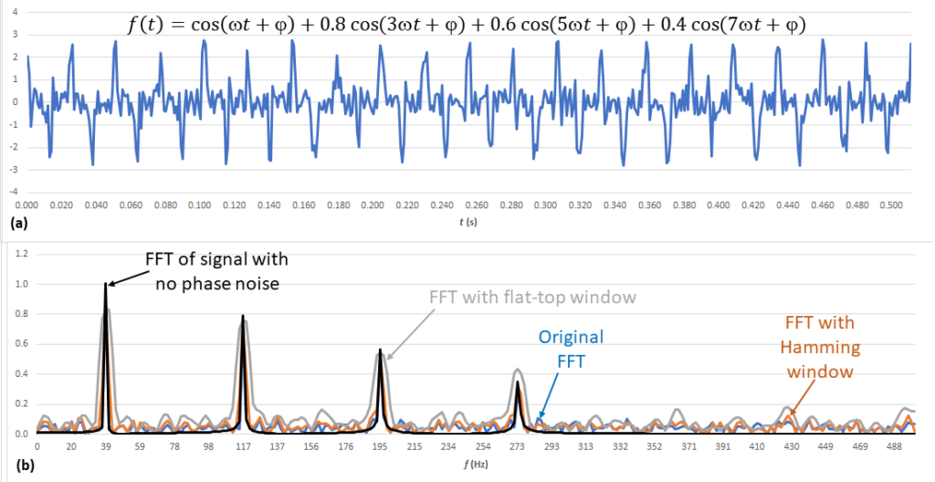
Figure 1a shows the original time-domain signal and the equation that defines it, where ω= 2π(39.1 Hz) and φ represents phase noise. To calculate φ, I used this Excel equation:

φ = -0.5+RAND()

RAND returns a random value between 0 and 1, so the expression returns a random value between -0.5 and +0.5, representing 1-radian peak-to-peak random phase noise. Figure 1b repeats Figure 8 from Part 3 but adds a transform (black trace) of the signal without phase noise, which has the expected amplitudes. The problem was not a spectral leakage problem that windowing could solve but rather an actual signal impairment in the form of phase noise.

Figure 1. A sample signal (a) yields the black FFT trace (b) when j = 0.

Can the FFT measure the phase noise?

The Excel FFT is not a great tool for that, which can be addressed using techniques discussed in an earlier series on phase noise (see part 1 and part 2). But the FFT can measure phase angle: the arctangent of the ratio of the imaginary to real parts of the complex FFT.

That seems easy.

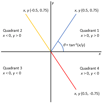
Be careful. Consider the blue vector in Figure 2. The phase angle θ is the arctangent of 0.75/0.5 = 1.5, and you can use the Excel ATAN() function to correctly find θ= 56.3°. But try the same approach for the orange vector. Your answer will be -56.3° (the red vector) instead of the expected 123.7°.

Figure 2. Keep track of quadrants when calculating q.

What causes that?
Once you calculate the ratio, you’ve stripped out information about how x and y individually contribute to the quotient’s polarity. For example, 0.75/-0.5 (quadrant 2) and -0.75/0.5 (quadrant 4) both equal -1.5 and ATAN() defaults to quadrant 4. To compensate, we could add some conditional programming steps: “If x < 0 and y > 0, then quadrant 2,” for example. Fortunately, Excel includes the ATAN2(x,y) function, which does that for us.

How do we modify our spreadsheet to calculate phase?

To add phase calculation to the Figure 4 spreadsheet in part 2, follow the steps in red in Figure 3.

Figure 3. Follow the steps in red to add phase calculation to the FFT.

Applying the Figure 4a sample waveform as the FFT input, we plot the Figure 4b FFT magnitude and phase — with the latter about 2.42 radians, or 139°, at 39.1 Hz.

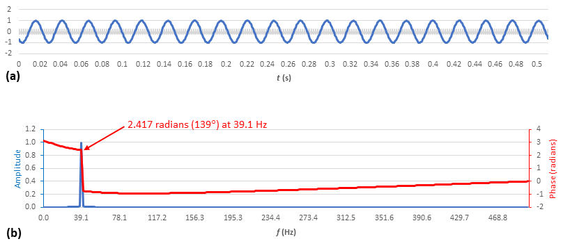
Figure 4. The FFT of a sample waveform (a) result in an amplitude and phase plot (b).

Woah! I can buy 139° at 39.1 Hz. But what is going on with the rest of that phase plot?

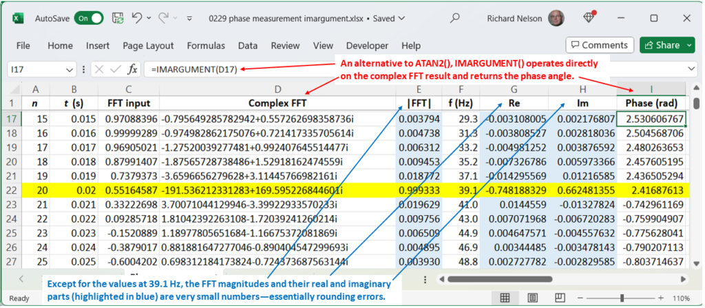
Let’s take another look at the spreadsheet and scroll down to 39.1 Hz (highlighted in yellow in Figure 5). At any other frequency, the real and imaginary parts of the complex FFT should be zero, and the FFT would return a divide-by-zero error. However, the numbers (highlighted in blue) are small but not zero. We are essentially taking the arctangents of ratios of rounding errors and getting meaningless results.

Figure 5. Except for the values at 39.1 Hz (yellow), the FFT’s magnitude and real and imaginary parts are very small numbers (blue).

A way to “clean up” the plot is to use an IF statement to plot zeros when the imaginary part falls below a certain threshold (Figure 6). Of course, the phase is not zero. Phase requires periodic changes in magnitude, and if those are not present (for example, any DC level, including zero), phase has no meaning.

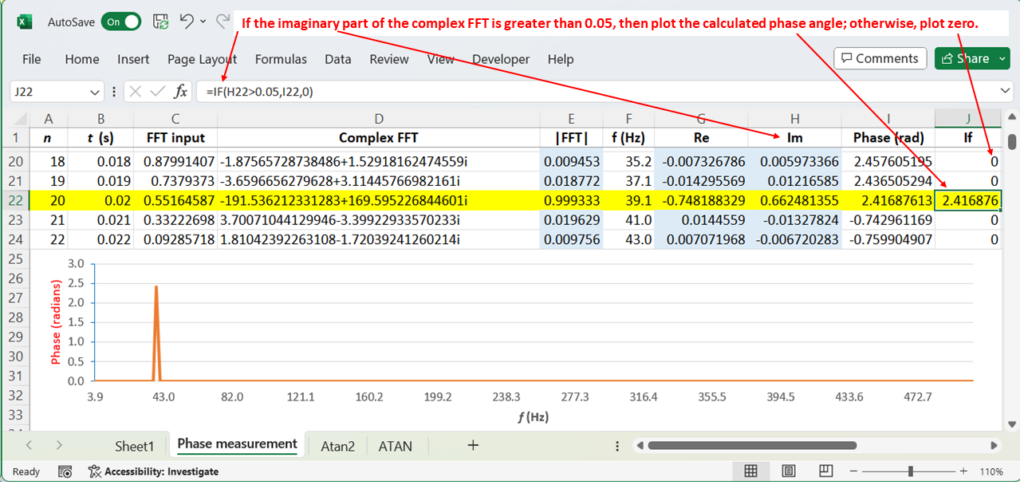
Figure 6. An IF statement plots invalid phase calculations as zero.

Also, notice a change I made in Figure 5. In column I, I replaced ATAN2() with IMARGUMENT(), which directly operates on a complex number and calculates the phase angle without the need to extract the real and imaginary parts.

Could you review what we’ve covered in this series?
Sure. In part 1, we reviewed the discrete Fourier transform and began setting up an Excel spreadsheet to run the FFT. In part 2, we completed the spreadsheet and ran an FFT on a signal resembling Figure 1b. In part 3, we investigated spectral leakage and windowing, and here, in part 4, we looked at phase.
What’s a key takeaway?
Excel presents an interesting way of learning about the FFT, but your best bet for professional work is commercial engineering software or the FFT tool that comes with your oscilloscope. Let me also refer you to NumPy, a Python-based open-source project for scientific computing. It offers several FFT and other transform algorithms for further exploration.